11 God Spiked the Integers

Load the packages.

# Load
library(tidyverse)
library(tidybayes)
library(rstan)
library(loo)
library(patchwork)
library(posterior)

# Drop grid lines
theme_set(
  theme_gray() +
    theme(panel.grid = element_blank())
)

11.1 Binomial regression

11.1.1 Logistic regression: Prosocial chimpanzees.

Load the Silk et al. (2005) chimpanzees data.

data(chimpanzees, package = "rethinking")
d <- chimpanzees
rm(chimpanzees)

Make the index variable treatment, a variant of which we’ll be saving as a factor with labeled levels named labels.

d <- d |> 
  mutate(treatment = factor(1 + prosoc_left + 2 * condition)) |> 
  # This will come in handy, later
  mutate(labels = factor(treatment,
                         levels = 1:4,
                         labels = c("r/n", "l/n", "r/p", "l/p")))

We can use the count() function to get a sense of the distribution of the conditions in the data.

d |> 
  count(prosoc_left, condition, treatment, labels)

  prosoc_left condition treatment labels   n
1           0         0         1    r/n 126
2           0         1         3    r/p 126
3           1         0         2    l/n 126
4           1         1         4    l/p 126

We start with the simple intercept-only logistic regression model, which follows the statistical formula

\[ \begin{align*} \text{pulled-left}_i & \sim \operatorname{Binomial}(1, p_i) \\ \operatorname{logit}(p_i) & = \alpha \\ \alpha & \sim \operatorname{Normal}(0, w), \end{align*} \]

where \(w\) is the hyperparameter for \(\sigma\) the value for which we have yet to choose.

Make the stan_data with the compose_data() function.

# Make a data set for predictions
d_pred <- d |> 
  distinct(actor, prosoc_left, condition, treatment, labels)

# print(d_pred)

# Make the primary data list
stan_data <- d |> 
  select(actor, treatment, pulled_left) |> 
  compose_data(
  n_actor = n_distinct(actor),
  n_treatment = n_distinct(treatment),
  # For predictions
  n_pred = nrow(d_pred),
  pred_actor = d_pred$actor,
  pred_treatment = d_pred$treatment)

# What?
str(stan_data)

List of 10
 $ actor           : int [1:504(1d)] 1 1 1 1 1 1 1 1 1 1 ...
 $ treatment       : num [1:504(1d)] 1 1 2 1 2 2 2 2 1 1 ...
 $ n_treatment     : int 4
 $ pulled_left     : int [1:504(1d)] 0 1 0 0 1 1 0 0 0 0 ...
 $ n               : int 504
 $ n_actor         : int 7
 $ n_pred          : int 28
 $ pred_actor      : int [1:28] 1 1 1 1 2 2 2 2 3 3 ...
 $ pred_treatment  : num [1:28] 1 2 3 4 2 1 3 4 1 2 ...
 $ n_pred_treatment: int 4

Define and sample from the initial program for the prior simulations. Note how for this application, we don’t even need a data block in the model_code.

model_code_11.1 <- '
parameters {
  real a;
}
model {
  // Prior only
  a ~ normal(0, 10);
}
'

m11.1 <- stan(
  model_code = model_code_11.1, 
  data = stan_data,
  cores = 4, seed = 11)

Here’s Figure 11.3.a.

set.seed(11)

p1 <- data.frame(a = c(
  as_draws_df(m11.1) |> pull(a),
  rnorm(n = 4e3, mean = 0, sd = 1.5))) |> 
  mutate(p = plogis(a),
         omega = rep(c(10, 1.5), each = n() / 2) |> 
           as.character()) |> 
  
  ggplot(aes(x = p, color = omega, fill = omega)) +
  geom_density(adjust = 1/10, alpha = 1/2) +
  scale_color_discrete(expression(omega)) +
  scale_fill_discrete(expression(omega)) +
  labs(x = expression(italic(p)),
       subtitle = expression("a ~ Normal(0, "*omega*")"))

# What?
p1

Here we make the model_code for m11.2, and compile the prior predictive distribution with stan().

model_code_11.2 <- '
data {
  int<lower=1> n_treatment;
}
parameters {
  real a;
  vector[n_treatment] b;
}
model {
  // Priors only
  a ~ normal(0, 1.5);
  b ~ normal(0, 10);
}
'

m11.2 <- stan(
  model_code = model_code_11.2, 
  data = stan_data,
  cores = 4, seed = 11)

Note that this model would typically have identification issues. But since we’re just sampling from the prior, it isn’t an issue for now.

Here’s m11.3, which is also just for prior-predictive draws, but this time using \(\beta_{[1:4]} \sim \mathcal N(0, 0.5)\).

model_code_11.3 <- '
data {
  int<lower=1> n_treatment;
}
parameters {
  real a;
  vector[n_treatment] b;
}
model {
  a ~ normal(0, 1.5);
  b ~ normal(0, 0.5);  // This is the only new part
}
'

m11.3 <- stan(
  model_code = model_code_11.3, 
  data = stan_data,
  cores = 4, seed = 11)

Here we compute the probability difference estimand \(p_1 - p_2\) from the prior predictive distribution of m11.2 and m11.3, and save the results as prior_m11.2_df and prior_m11.3_df.

prior_m11.2_df <- m11.2 |> 
  spread_draws(a, b[treatment]) |> 
  filter(treatment < 3) |> 
  mutate(p = plogis(a + b)) |> 
  compare_levels(p, by = treatment)

prior_m11.3_df <- m11.3 |> 
  spread_draws(a, b[treatment]) |> 
  filter(treatment < 3) |> 
  mutate(p = plogis(a + b)) |> 
  compare_levels(p, by = treatment)

# What?
head(prior_m11.2_df)

# A tibble: 6 × 5
# Groups:   treatment [1]
  .chain .iteration .draw treatment        p
   <int>      <int> <int> <chr>        <dbl>
1      1          1     1 2 - 1     -0.0357 
2      1          2     2 2 - 1     -0.831  
3      1          3     3 2 - 1     -1.00   
4      1          4     4 2 - 1     -0.00966
5      1          5     5 2 - 1     -1.00   
6      1          6     6 2 - 1     -1.00

head(prior_m11.3_df)

# A tibble: 6 × 5
# Groups:   treatment [1]
  .chain .iteration .draw treatment       p
   <int>      <int> <int> <chr>       <dbl>
1      1          1     1 2 - 1     -0.147 
2      1          2     2 2 - 1      0.385 
3      1          3     3 2 - 1     -0.311 
4      1          4     4 2 - 1     -0.0233
5      1          5     5 2 - 1     -0.301 
6      1          6     6 2 - 1      0.0159

Now we combine the two to make Figure 11.3.b.

p2 <- bind_rows(prior_m11.2_df, prior_m11.3_df) |> 
  mutate(psi = rep(c(10, 0.5), each = n() / 2) |> 
           as.character()) |> 
  
  ggplot(aes(x = abs(p), color = psi, fill = psi)) +
  geom_density(adjust = 1/10, alpha = 1/2) +
  scale_color_discrete(expression(psi)) +
  scale_fill_discrete(expression(psi)) +
  labs(x = expression(abs(italic(p)[1]-italic(p)[2])),
       subtitle = expression("b ~ Normal(0, "*psi*")"))

# Combine
p1 | p2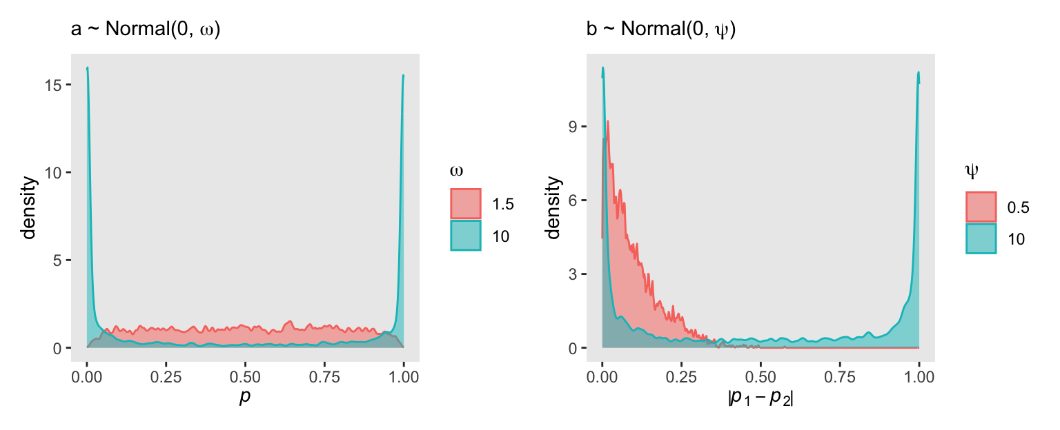

The average absolute prior difference is about 0.1, very similar to McElreath’s value from R code 11.9.

prior_m11.3_df |> 
  ungroup() |> 
  summarise(mean = abs(p) |> mean())

# A tibble: 1 × 1
    mean
   <dbl>
1 0.0963

The full model follows the form

\[ \begin{align*} \text{pulled-left}_i & \sim \operatorname{Binomial}(1, p_i) \\ \operatorname{logit}(p_i) & = \alpha_{\text{actor}[i]} + \beta_{\text{treatment}[i]} \\ \alpha_j & \sim \operatorname{Normal}(0, 1.5) \\ \beta_k & \sim \operatorname{Normal}(0, 0.5), \end{align*} \]

where we now have four levels of \(\alpha_j\), and seven levels of \(\beta_k\). We’ll call this model m11.4, and this time we actually sample from the posterior. In the generated quantities block, we’re defining a vector of predicted values p, as well as the log_lik values for information criteria.

model_code_11.4 <- '
data {
  int<lower=1> n;                       
  int<lower=1> n_actor;
  int<lower=1> n_treatment;
  int<lower=1> n_pred;
  array[n] int actor;
  array[n] int treatment;
  array[n_pred] int pred_actor;
  array[n_pred] int pred_treatment;
  array[n] int<lower=0, upper=1> pulled_left;
}
parameters {
  vector[n_actor] a;
  vector[n_treatment] b;
}
model {
  pulled_left ~ binomial(1, inv_logit(a[actor] + b[treatment]));
  a ~ normal(0, 1.5);
  b ~ normal(0, 0.5);
}
generated quantities {
  vector[n_pred] p;
  vector[n] log_lik;
  
  p = inv_logit(a[pred_actor] + b[pred_treatment]);
  for (i in 1:n) log_lik[i] = binomial_lpmf(pulled_left[i] | 1, inv_logit(a[actor[i]] + b[treatment[i]]));
}
'

m11.4 <- stan(
  model_code = model_code_11.4, 
  data = stan_data,
  cores = 4, seed = 11)

Check the model summary.

print(m11.4, pars = c("a", "b"), probs = c(0.055, 0.945))

Inference for Stan model: anon_model.
4 chains, each with iter=2000; warmup=1000; thin=1; 
post-warmup draws per chain=1000, total post-warmup draws=4000.

      mean se_mean   sd  5.5% 94.5% n_eff Rhat
a[1] -0.45    0.01 0.32 -0.96  0.07  1195    1
a[2]  3.90    0.01 0.77  2.75  5.20  2919    1
a[3] -0.75    0.01 0.34 -1.29 -0.21  1232    1
a[4] -0.75    0.01 0.34 -1.28 -0.20  1248    1
a[5] -0.45    0.01 0.33 -0.97  0.08  1176    1
a[6]  0.47    0.01 0.33 -0.04  1.02  1115    1
a[7]  1.96    0.01 0.41  1.31  2.64  1412    1
b[1] -0.04    0.01 0.29 -0.50  0.43   954    1
b[2]  0.48    0.01 0.29  0.02  0.93  1038    1
b[3] -0.38    0.01 0.29 -0.85  0.06  1033    1
b[4]  0.37    0.01 0.29 -0.09  0.82  1100    1

Samples were drawn using NUTS(diag_e) at Thu Aug 15 11:27:49 2024.
For each parameter, n_eff is a crude measure of effective sample size,
and Rhat is the potential scale reduction factor on split chains (at 
convergence, Rhat=1).

Here’s the coefficient plot for the intercepts, transformed onto the probability scale.

m11.4 |> 
  spread_draws(a[j]) |> 
  mutate(j = factor(j, levels = 7:1)) |> 
  
  ggplot(aes(x = plogis(a), y = j)) +
  stat_pointinterval(point_interval = mean_qi, .width = 0.89, 
                     linewidth = 1, shape = 1) +
  xlim(0:1) +
  ylab(expression(italic(j)))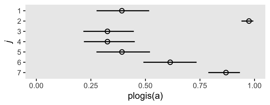

Here’s the coefficient plot for the treatment parameters, on the log-odds scale.

m11.4 |> 
  spread_draws(b[k]) |> 
  left_join(d |> 
              distinct(treatment, labels) |> 
              mutate(k = as.integer(treatment)),
            by = join_by(k)) |>
  mutate(labels = fct_rev(labels)) |> 
  
  ggplot(aes(x = b, y = labels)) +
  stat_pointinterval(point_interval = mean_qi, .width = 0.89, 
                     linewidth = 1, shape = 1) +
  ylab(NULL)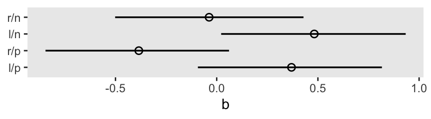

Here are the two contrasts.

m11.4 |> 
  spread_draws(b[k]) |> 
  pivot_wider(names_from = k, values_from = b) |> 
  mutate(db13 = `1` - `3`,
         db24 = `2` - `4`) |> 
  pivot_longer(starts_with("db")) |> 
  mutate(name = fct_rev(name)) |> 
  
  ggplot(aes(x = value, y = name)) +
  stat_pointinterval(point_interval = mean_qi, .width = 0.89, 
                     linewidth = 1, shape = 1) +
  ylab(NULL)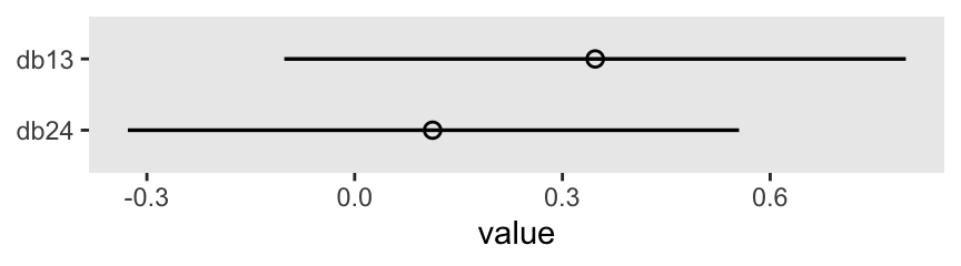

Next, we prepare for the posterior predictive check. McElreath showed how to compute empirical proportions by the levels of actor and treatment with the by() function. Our approach will be with a combination of group_by() and summarise(). Here’s what that looks like for actor == 1.

d |>
  group_by(actor, treatment) |>
  summarise(proportion = mean(pulled_left)) |> 
  filter(actor == 1)

# A tibble: 4 × 3
# Groups:   actor [1]
  actor treatment proportion
  <int> <fct>          <dbl>
1     1 1              0.333
2     1 2              0.5  
3     1 3              0.278
4     1 4              0.556

Now we’ll follow that through to make the top panel of Figure 11.4.

# Wrangle
p1 <- d |>
  group_by(actor, treatment) |>
  summarise(p = mean(pulled_left)) |> 
  left_join(d |> distinct(actor, treatment, labels, condition, prosoc_left),
            by = c("actor", "treatment")) |> 
  mutate(actor = str_c("actor ", actor),
         condition = factor(condition)) |> 
  
  # Plot
  ggplot(aes(x = labels, y = p)) +
  geom_hline(yintercept = 0.5, color = "white") +
  geom_line(aes(group = prosoc_left),
            linewidth = 1/4) +
  geom_point(aes(color = condition),
             size = 2.5, show.legend = F) + 
  scale_x_discrete(NULL, breaks = NULL) +
  facet_grid("observed proportions" ~ actor)
  
# Display
p1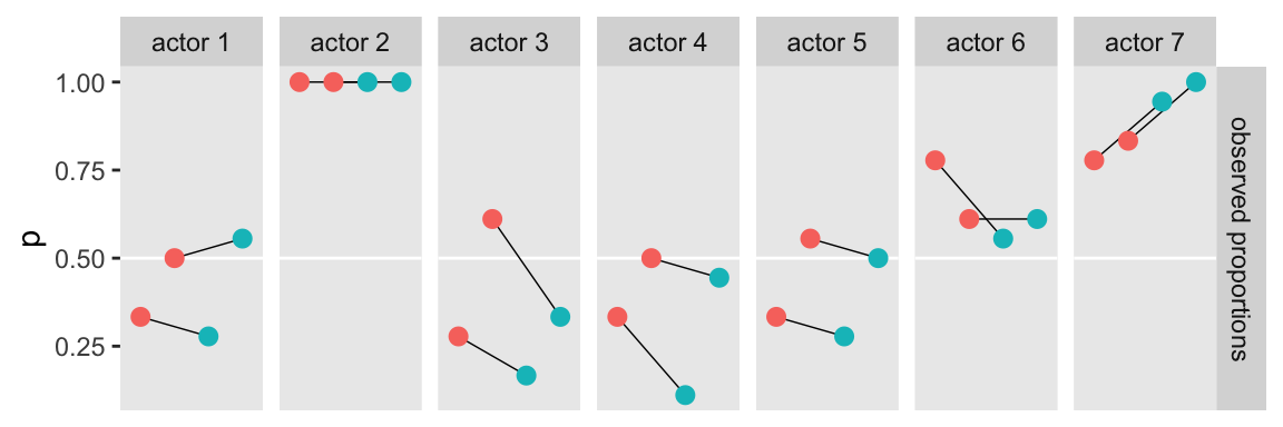

Make the bottom panel of Figure 11.4. Note how we’re using our p parameters for this plow, which we defined in the generated quantities block, above.

# Wrangle
p2 <- m11.4 |> 
  spread_draws(p[i]) |> 
  left_join(d_pred |> 
              mutate(i = 1:n()),
            by = join_by(i)) |> 
  mutate(actor = str_c("actor ", actor),
         condition = factor(condition)) |> 
  group_by(actor, prosoc_left, condition, treatment, labels) |> 
  mean_qi(p, .width = 0.89) |> 
  
  # Plot
  ggplot(aes(x = labels, y = p)) +
  geom_hline(yintercept = .5, color = "white") +
  geom_line(aes(group = prosoc_left),
            linewidth = 1/4) +
  geom_pointinterval(aes(ymin = .lower, ymax = .upper, fill = condition),
                     linewidth = 1, shape = 21) +
  scale_fill_discrete(breaks = NULL) +
  facet_grid("posterior predictions" ~ actor) +
  theme(strip.text.x = element_blank())

# Display
p2

Combine the two panels to make the full Figure 11.4.

(p1 / p2) &
  scale_y_continuous("proportion left lever", 
                     breaks = 0:2 / 2, limits = 0:1)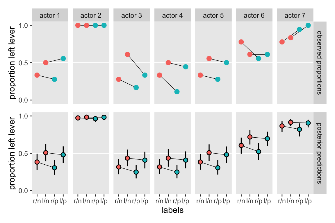

Let’s make two more index variables.

d <- d |> 
  mutate(side = prosoc_left + 1,  # right 1, left 2
         cond = condition + 1)    # no partner 1, partner 2

# What?
d |> 
  distinct(prosoc_left, condition, side, cond)

  prosoc_left condition side cond
1           0         0    1    1
2           1         0    2    1
3           0         1    1    2
4           1         1    2    2

Update the stan_data.

stan_data <- d |> 
  select(actor, side, cond, pulled_left) |> 
  compose_data(
  n_actor = n_distinct(actor),
  n_side = n_distinct(side),
  n_cond = n_distinct(cond))

# What?
str(stan_data)

List of 8
 $ actor      : int [1:504(1d)] 1 1 1 1 1 1 1 1 1 1 ...
 $ side       : num [1:504(1d)] 1 1 2 1 2 2 2 2 1 1 ...
 $ cond       : num [1:504(1d)] 1 1 1 1 1 1 1 1 1 1 ...
 $ pulled_left: int [1:504(1d)] 0 1 0 0 1 1 0 0 0 0 ...
 $ n          : int 504
 $ n_actor    : int 7
 $ n_side     : int 2
 $ n_cond     : int 2

Next we define the new model_code and fit m11.5. In the model block, note we’re using the binomial_logit() function for the likelihood, rather than the binomial() function, as in the last few models. As we covered back in Section 1.3.3, sometimes Stan provides variants of popular likelihood functions parameterized in terms of their typical link functions. By using the binomial_logit() function, we don’t need to nest the linear model within the inv_logit() function. The logit link is presumed. In a similar way, we have used the binomial_logit_lpmf() within the generated quantities block, rather than the binomial_lpmf() function. Both methods work just fine. In this case, the binomial_logit() function resulted in a faster computation time, and slightly better ESS diagnostics.

model_code_11.5 <- '
data {
  int<lower=1> n;                       
  int<lower=1> n_actor;
  int<lower=1> n_side;
  int<lower=1> n_cond;
  array[n] int actor;
  array[n] int side;
  array[n] int cond;
  array[n] int<lower=0, upper=1> pulled_left;
}
parameters {
  vector[n_actor] a;
  vector[n_side] b1;
  vector[n_cond] b2;
}
model {
  pulled_left ~ binomial_logit(1, a[actor] + b1[side] + b2[cond]);
  // This also works
  // pulled_left ~ binomial(1, inv_logit(a[actor] + b1[side] + b2[cond]));
  a ~ normal(0, 1.5);
  b1 ~ normal(0, 0.5);
  b2 ~ normal(0, 0.5);
}
generated quantities {
  vector[n] eta;  // To simplify the `log_lik` code
  vector[n] log_lik;
  
  eta = a[actor] + b1[side] + b2[cond];
  for (i in 1:n) log_lik[i] = binomial_logit_lpmf(pulled_left[i] | 1, eta[i]);
  // This also works
  // for (i in 1:n) log_lik[i] = binomial_lpmf(pulled_left[i] | 1, inv_logit(eta[i]));
  
  // This also works for the `log_lik`, and it negates the need for `eta` from above
  // for (i in 1:n) log_lik[i] = binomial_lpmf(pulled_left[i] | 1, inv_logit(a[actor[i]] + b1[side[i]] + b2[cond[i]]));
}
'

m11.5 <- stan(
  model_code = model_code_11.5, 
  data = stan_data,
  cores = 4, seed = 11)

Check the model summary.

print(m11.5, pars = c("a", "b1", "b2"), probs = c(0.055, 0.945))

Inference for Stan model: anon_model.
4 chains, each with iter=2000; warmup=1000; thin=1; 
post-warmup draws per chain=1000, total post-warmup draws=4000.

       mean se_mean   sd  5.5% 94.5% n_eff Rhat
a[1]  -0.63    0.01 0.44 -1.33  0.07  1259    1
a[2]   3.77    0.02 0.79  2.58  5.13  1923    1
a[3]  -0.94    0.01 0.44 -1.65 -0.22  1377    1
a[4]  -0.93    0.01 0.44 -1.64 -0.24  1349    1
a[5]  -0.64    0.01 0.44 -1.35  0.06  1296    1
a[6]   0.29    0.01 0.44 -0.42  0.99  1349    1
a[7]   1.78    0.01 0.50  0.97  2.56  1573    1
b1[1] -0.19    0.01 0.34 -0.74  0.36  1469    1
b1[2]  0.50    0.01 0.34 -0.04  1.04  1453    1
b2[1]  0.27    0.01 0.33 -0.25  0.81  1487    1
b2[2]  0.02    0.01 0.33 -0.49  0.55  1502    1

Samples were drawn using NUTS(diag_e) at Thu Sep 12 13:47:39 2024.
For each parameter, n_eff is a crude measure of effective sample size,
and Rhat is the potential scale reduction factor on split chains (at 
convergence, Rhat=1).

Compare the two models by the LOO with the extract_log_lik() and loo_compare() functions.

loo_compare(
  extract_log_lik(m11.4) |> loo(),
  extract_log_lik(m11.5) |> loo()
) |> 
  print(simplify = FALSE)

       elpd_diff se_diff elpd_loo se_elpd_loo p_loo  se_p_loo looic  se_looic
model2    0.0       0.0  -265.3      9.6         7.7    0.4    530.6   19.1  
model1   -0.6       0.7  -265.9      9.5         8.3    0.4    531.8   18.9

11.1.1.1 Overthinking: Adding log-probability calculations to a Stan model.

We did this with m11.5, above.

11.1.2 Relative shark and absolute deer.

Based on the full model, m11.4, here’s how you might compute the posterior mean and 89% intervals for the proportional odds of switching from treatment == 2 to treatment == 4.

as_draws_df(m11.4) |> 
  mutate(proportional_odds = exp(`b[4]` - `b[2]`)) |> 
  mean_qi(proportional_odds, .width = 0.89)

# A tibble: 1 × 6
  proportional_odds .lower .upper .width .point .interval
              <dbl>  <dbl>  <dbl>  <dbl> <chr>  <chr>    
1             0.929  0.574   1.39   0.89 mean   qi

A limitation of relative measures measures like proportional odds is they ignore what you might think of as the reference or the baseline.

11.1.2.1 Overthinking: Proportional odds and relative risk.

11.1.3 Aggregated binomial: Chimpanzees again, condensed.

With the tidyverse, we can use group_by() and summarise() to achieve what McElreath did with aggregate().

d_aggregated <- d |>
  group_by(treatment, actor, side, cond) |>
  summarise(left_pulls = sum(pulled_left)) |> 
  ungroup()

# What?
d_aggregated |>
  head(n = 10)

# A tibble: 10 × 5
   treatment actor  side  cond left_pulls
   <fct>     <int> <dbl> <dbl>      <int>
 1 1             1     1     1          6
 2 1             2     1     1         18
 3 1             3     1     1          5
 4 1             4     1     1          6
 5 1             5     1     1          6
 6 1             6     1     1         14
 7 1             7     1     1         14
 8 2             1     2     1          9
 9 2             2     2     1         18
10 2             3     2     1         11

Update the stan_data for the new d_aggregated format.

stan_data <- d_aggregated |> 
  compose_data(n_actor = n_distinct(d_aggregated$actor))

# What?
str(stan_data)

List of 8
 $ treatment  : num [1:28(1d)] 1 1 1 1 1 1 1 2 2 2 ...
 $ n_treatment: int 4
 $ actor      : int [1:28(1d)] 1 2 3 4 5 6 7 1 2 3 ...
 $ side       : num [1:28(1d)] 1 1 1 1 1 1 1 2 2 2 ...
 $ cond       : num [1:28(1d)] 1 1 1 1 1 1 1 1 1 1 ...
 $ left_pulls : int [1:28(1d)] 6 18 5 6 6 14 14 9 18 11 ...
 $ n          : int 28
 $ n_actor    : int 7

Define model_code_11.6 and fit the model. As an alternative, try fitting the model with the binomial_logit() and binomial_logit_lpmf() functions like we did for m11.5, above. Which method has better HMC chain diagnostics?

model_code_11.6 <- '
data {
  int<lower=1> n;
  int<lower=1> n_actor;
  int<lower=1> n_treatment;
  array[n] int treatment;
  array[n] int actor;
  array[n] int<lower=0, upper=18> left_pulls;
}
parameters {
  vector[n_actor] a;
  vector[n_treatment] b;
}
model {
  left_pulls ~ binomial(18, inv_logit(a[actor] + b[treatment]));
  // left_pulls ~ binomial_logit(18, a[actor] + b[treatment]);
  a ~ normal(0, 1.5);
  b ~ normal(0, 0.5);
}
generated quantities {
  vector[n] eta;
  vector[n] log_lik;
  eta = a[actor] + b[treatment];
  for (i in 1:n) log_lik[i] = binomial_lpmf(left_pulls[i] | 18, inv_logit(eta[i]));
  // for (i in 1:n) log_lik[i] = binomial_logit_lpmf(left_pulls[i] | 18, eta[i]);
}
'

m11.6 <- stan(
  model_code = model_code_11.6, 
  data = stan_data,
  cores = 4, seed = 11)

Rather than the typical print() summary, here we’ll compare the a and b parameters in this aggregated binomial model m11.6 with its disaggregated version m11.4 in a coefficient plot.

bind_rows(
  as_draws_df(m11.4) |> 
    select(.draw, `a[1]`:`b[4]`) ,
  as_draws_df(m11.6) |> 
    select(.draw, `a[1]`:`b[4]`) 
) |> 
  mutate(type = rep(c("disaggregated", "aggregated"), each = n() / 2)) |> 
  pivot_longer(`a[1]`:`b[4]`) |> 
  mutate(class = str_extract(name, "\\w")) |> 
  
  ggplot(aes(x = value, y = name,
             color = type)) +
  stat_pointinterval(.width = 0.89, linewidth = 1, shape = 1,
                     position = position_dodge(width = -0.5)) +
  scale_y_discrete(NULL, labels = ggplot2:::parse_safe) +
  xlab("posterior") +
  facet_wrap(~ class, scales = "free")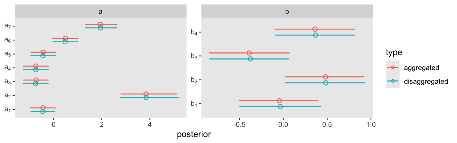

Different version of the likelihood, same model. Feed the extract_log_lik() results into loo(), and save output as loo_m11.6.

loo_m11.6 <- extract_log_lik(m11.6) |>
  loo()

Warning: Some Pareto k diagnostic values are too high. See help('pareto-k-diagnostic') for details.

# What?
print(loo_m11.6)


Computed from 4000 by 28 log-likelihood matrix.

         Estimate  SE
elpd_loo    -57.1 4.2
p_loo         8.4 1.5
looic       114.1 8.4
------
MCSE of elpd_loo is NA.
MCSE and ESS estimates assume independent draws (r_eff=1).

Pareto k diagnostic values:
                         Count Pct.    Min. ESS
(-Inf, 0.7]   (good)     27    96.4%   407     
   (0.7, 1]   (bad)       1     3.6%   <NA>    
   (1, Inf)   (very bad)  0     0.0%   <NA>    
See help('pareto-k-diagnostic') for details.

Unlike with McElreath’s compare() code in the text, the loo::loo_compare() will not let us directly compare the two versions of the model. I’m going to supress the output, but if you execute this code on your computer, you’ll see it returns a warning.

loo_compare(
  extract_log_lik(m11.4) |> loo(),
  loo_m11.6
) |> 
  print(simplify = FALSE)

To understand what’s going on, consider how you might describe six 1’s out of nine trials in the aggregated form,

\[\Pr(6|9, p) = \frac{6!}{6!(9 - 6)!} p^6 (1 - p)^{9 - 6}.\]

If we still stick with the same data, but this time re-express those as nine dichotomous data points, we now describe their joint probability as

\[\Pr(1, 1, 1, 1, 1, 1, 0, 0, 0 \mid p) = p^6 (1 - p)^{9 - 6}.\]

Let’s work this out in code.

# Deviance of aggregated 6-in-9 
-2 * dbinom(6, size = 9, prob = 0.2, log = TRUE)

[1] 11.79048

# Deviance of dis-aggregated 
-2 * sum(dbinom(c(1, 1, 1, 1, 1, 1, 0, 0, 0), size = 1, prob = 0.2, log = TRUE))

[1] 20.65212

But this difference is entirely meaningless. It is just a side effect of how we organized the data. The posterior distribution for the probability of success on each trial will end up the same, either way. (p. 339)

This is what our coefficient plot showed us, above. The posterior distribution was the same within simulation variance for m11.4 and m11.6. Just like McElreath reported in the text, we also got a warning about high Pareto \(k\) values from the aggregated binomial model, m11.6. To access the message and its associated table directly, we can feed our loo_m11.6 object into the loo::pareto_k_table function.

loo_m11.6 |> 
  loo::pareto_k_table()

Pareto k diagnostic values:
                         Count Pct.    Min. ESS
(-Inf, 0.7]   (good)     27    96.4%   407     
   (0.7, 1]   (bad)       1     3.6%   <NA>    
   (1, Inf)   (very bad)  0     0.0%   <NA>

11.1.4 Aggregated binomial: Graduate school admissions.

Load the infamous UCBadmit data.

data(UCBadmit, package = "rethinking")
d <- UCBadmit
rm(UCBadmit)

# What?
print(d)

   dept applicant.gender admit reject applications
1     A             male   512    313          825
2     A           female    89     19          108
3     B             male   353    207          560
4     B           female    17      8           25
5     C             male   120    205          325
6     C           female   202    391          593
7     D             male   138    279          417
8     D           female   131    244          375
9     E             male    53    138          191
10    E           female    94    299          393
11    F             male    22    351          373
12    F           female    24    317          341

Now compute our new index variable, gid. Notice that if we save gid as a factor, the compose_data() a couple blocks below will automatically compute n_gid. We’ll also slip in a case variable that saves the row numbers as a factor, which will come in handy later when we plot.

d <- d |>  
  mutate(gid  = ifelse(applicant.gender == "male", 1, 2) |> factor(),
         case = 1:n() |> factor())

# What?
d |> 
  distinct(applicant.gender, gid)

  applicant.gender gid
1             male   1
2           female   2

The univariable logistic model with male as the sole predictor of admit follows the form

\[ \begin{align*} \text{admit}_i & \sim \operatorname{Binomial}(n_i, p_i) \\ \text{logit}(p_i) & = \alpha_{\text{gid}[i]} \\ \alpha_j & \sim \operatorname{Normal}(0, 1.5), \end{align*} \]

where \(n_i = \text{applications}_i\), the rows are indexed by \(i\), and the two levels of \(\text{gid}\) are indexed by \(j\).

Make the stan_data with the compose_data() function.

stan_data <- d |> 
  select(dept, gid, admit, applications) |>
  compose_data()

# What?
str(stan_data)

List of 7
 $ dept        : num [1:12(1d)] 1 1 2 2 3 3 4 4 5 5 ...
 $ n_dept      : int 6
 $ gid         : num [1:12(1d)] 1 2 1 2 1 2 1 2 1 2 ...
 $ n_gid       : int 2
 $ admit       : int [1:12(1d)] 512 89 353 17 120 202 138 131 53 94 ...
 $ applications: int [1:12(1d)] 825 108 560 25 325 593 417 375 191 393 ...
 $ n           : int 12

Make the model_code and fit m11.7 with stan(). Note the generated quantities block for the posterior-predictive check to come.

model_code_11.7 <- '
data {
  int<lower=1> n;
  int<lower=1> n_gid;
  array[n] int gid;
  array[n] int<lower=1> applications;
  array[n] int<lower=0> admit;
}
parameters {
  vector[n_gid] a;
}
model {
  admit ~ binomial(applications, inv_logit(a[gid]));
  a ~ normal(0, 1.5);
}
generated quantities {
  // For the pp check
  array[n] int<lower=0> pp_admit = binomial_rng(applications, inv_logit(a[gid]));
}
'

m11.7 <- stan(
  model_code = model_code_11.7, 
  data = stan_data,
  cores = 4, iter = 4000, seed = 11)

Check the model summary.

print(m11.7, pars = "a", probs = c(0.055, 0.945))

Inference for Stan model: anon_model.
4 chains, each with iter=4000; warmup=2000; thin=1; 
post-warmup draws per chain=2000, total post-warmup draws=8000.

      mean se_mean   sd  5.5% 94.5% n_eff Rhat
a[1] -0.22       0 0.04 -0.28 -0.16  5765    1
a[2] -0.83       0 0.05 -0.91 -0.75  5699    1

Samples were drawn using NUTS(diag_e) at Thu Aug 15 11:33:46 2024.
For each parameter, n_eff is a crude measure of effective sample size,
and Rhat is the potential scale reduction factor on split chains (at 
convergence, Rhat=1).

We’ll hold off on computing diff_a and diff_p, for a moment, and jump straight to Figure 11.5. Note how we’re using the pp_admit values we computed with the generated quantities block.

m11.7 |> 
  spread_draws(pp_admit[i]) |> 
  left_join(d |> 
              mutate(i = as.integer(case)),
            by = join_by(i)) |> 
  
  ggplot(aes(x = gid)) +
  stat_pointinterval(aes(y = pp_admit / applications),
                     .width = 0.89, linewidth = 1, shape = 1) +
  geom_point(data = d,
             aes(y = admit / applications),
             color = "blue") +
  geom_path(data = d,
             aes(y = admit / applications, group = dept),
             color = "blue") +
  scale_x_discrete(NULL, labels = c("male", "female")) +
  scale_y_continuous("admit", limits = 0:1) +
  facet_wrap(~ dept, nrow = 1)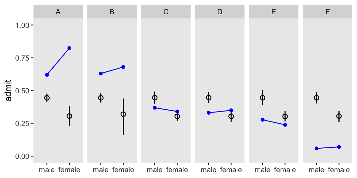

I should acknowledge I got the idea to reformat the plot this way from Arel-Bundock’s work.

Now we fit the model

\[ \begin{align*} \text{admit}_i & \sim \operatorname{Binomial} (n_i, p_i) \\ \text{logit}(p_i) & = \alpha_{\text{gid}[i]} + \delta_{\text{dept}[i]} \\ \alpha_j & \sim \operatorname{Normal} (0, 1.5) \\ \delta_k & \sim \operatorname{Normal} (0, 1.5), \end{align*} \]

where departments are indexed by \(k\). Make the model_code and fit m11.8 with stan(). Note how we’re increasing the iter argument in stan().

model_code_11.8 <- '
data {
  int<lower=1> n;
  int<lower=1> n_gid;
  int<lower=1> n_dept;
  array[n] int gid;
  array[n] int dept;
  array[n] int applications;
  array[n] int<lower=0> admit;
}
parameters {
  vector[n_gid] a;
  vector[n_dept] d;
}
model {
  admit ~ binomial(applications, inv_logit(a[gid] + d[dept]));
  a ~ normal(0, 1.5);
  d ~ normal(0, 1.5);
}
generated quantities {
  // For the pp check
  array[n] int<lower=0> pp_admit = binomial_rng(applications, inv_logit(a[gid] + d[dept]));
}
'

m11.8 <- stan(
  model_code = model_code_11.8, 
  data = stan_data,
  cores = 4, iter = 4000, seed = 11)

Check the model summary.

print(m11.8, pars = c("a", "d"), probs = c(0.055, 0.945))

Inference for Stan model: anon_model.
4 chains, each with iter=4000; warmup=2000; thin=1; 
post-warmup draws per chain=2000, total post-warmup draws=8000.

      mean se_mean   sd  5.5% 94.5% n_eff Rhat
a[1] -0.54    0.02 0.54 -1.42  0.34   603    1
a[2] -0.45    0.02 0.54 -1.33  0.44   607    1
d[1]  1.12    0.02 0.54  0.24  2.00   604    1
d[2]  1.08    0.02 0.55  0.18  1.96   603    1
d[3] -0.14    0.02 0.54 -1.02  0.74   611    1
d[4] -0.17    0.02 0.55 -1.05  0.71   610    1
d[5] -0.61    0.02 0.55 -1.51  0.28   623    1
d[6] -2.17    0.02 0.55 -3.07 -1.27   642    1

Samples were drawn using NUTS(diag_e) at Thu Aug 15 11:35:07 2024.
For each parameter, n_eff is a crude measure of effective sample size,
and Rhat is the potential scale reduction factor on split chains (at 
convergence, Rhat=1).

Here we’ll show the contrasts for the two models in a coefficient plot.

bind_rows(
  as_draws_df(m11.7) |> select(.draw, `a[1]`:`a[2]`),
  as_draws_df(m11.8) |> select(.draw, `a[1]`:`a[2]`)
) |> 
  mutate(fit = rep(c("m11.7", "m11.8"), each = n() / 2),
         diff_a = `a[1]` - `a[2]`,
         diff_p = plogis(`a[1]`) - plogis(`a[2]`)) |> 
  pivot_longer(contains("diff")) |> 
  
  ggplot(aes(x = value, y = name,
             color = fit)) +
  geom_vline(xintercept = 0, color = "white") +
  stat_pointinterval(.width = 0.89, linewidth = 1, shape = 1,
                     position = position_dodge(width = -0.5)) +
  labs(x = "contrast",
       y = NULL)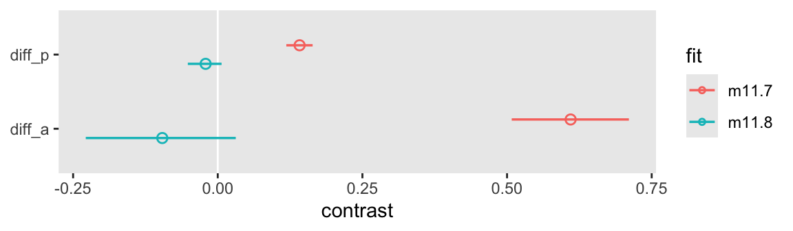

Here’s our tidyverse-style tabulation of the proportions of applicants in each department by gid.

d |> 
  group_by(dept) |> 
  mutate(proportion = applications / sum(applications)) |> 
  select(dept, gid, proportion) |> 
  pivot_wider(names_from = dept,
              values_from = proportion) |> 
  mutate_if(is.double, round, digits = 2)

# A tibble: 2 × 7
  gid       A     B     C     D     E     F
  <fct> <dbl> <dbl> <dbl> <dbl> <dbl> <dbl>
1 1      0.88  0.96  0.35  0.53  0.33  0.52
2 2      0.12  0.04  0.65  0.47  0.67  0.48

If we make another version of Figure 11.5 with m11.8, we’ll see conditioning on both substantially improved the posterior predictive distribution.

m11.8 |> 
  spread_draws(pp_admit[i]) |> 
  left_join(d |> 
              mutate(i = as.integer(case)),
            by = join_by(i)) |> 
  
  ggplot(aes(x = gid)) +
  stat_pointinterval(aes(y = pp_admit / applications),
                     .width = 0.89, linewidth = 1, shape = 1) +
  geom_point(data = d,
             aes(y = admit / applications),
             color = "blue") +
  geom_path(data = d,
             aes(y = admit / applications, group = dept),
             color = "blue") +
  scale_x_discrete(NULL, labels = c("male", "female")) +
  scale_y_continuous("admit", limits = 0:1) +
  facet_wrap(~ dept, nrow = 1)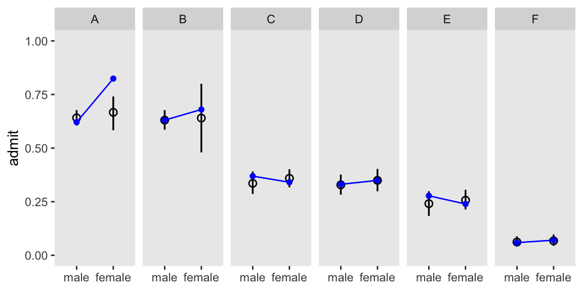

McElreath recommended we look at the pairs() plot to get a sense of how highly correlated the parameters in our m11.8 model are. Here’s the plot.

pairs(m11.8, pars = c("a", "d"), gap = 0.25)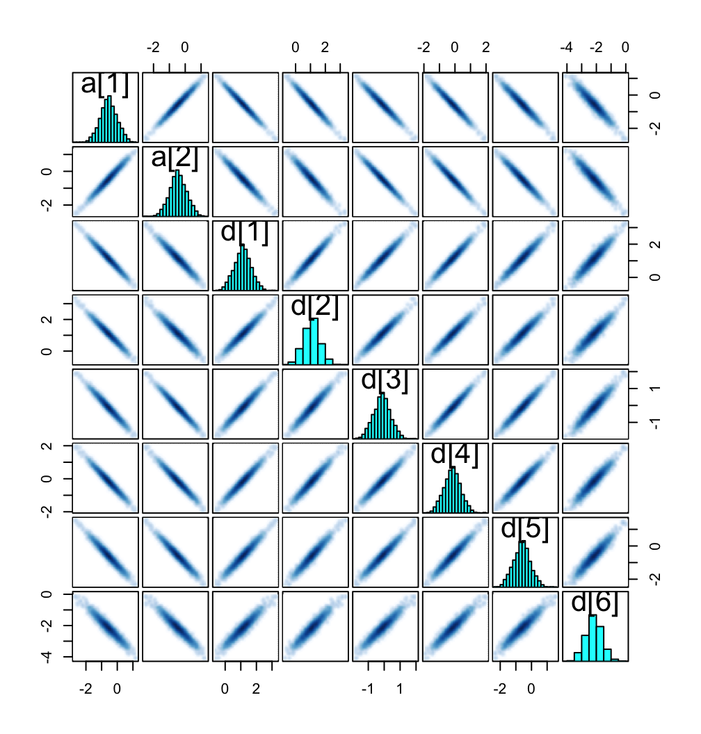

11.1.4.1 Rethinking: Simpson’s paradox is not a paradox.

11.2 Poisson regression

11.2.1 Example: Oceanic tool complexity.

Load the Kline data (see Kline & Boyd, 2010).

data(Kline, package = "rethinking")
d <- Kline
rm(Kline)

# What?
print(d)

      culture population contact total_tools mean_TU
1    Malekula       1100     low          13     3.2
2     Tikopia       1500     low          22     4.7
3  Santa Cruz       3600     low          24     4.0
4         Yap       4791    high          43     5.0
5    Lau Fiji       7400    high          33     5.0
6   Trobriand       8000    high          19     4.0
7       Chuuk       9200    high          40     3.8
8       Manus      13000     low          28     6.6
9       Tonga      17500    high          55     5.4
10     Hawaii     275000     low          71     6.6

Here are our new columns.

d <- d |>
  mutate(log_pop_std = (log(population) - mean(log(population))) / sd(log(population)),
         cid         = ifelse(contact == "high", "2", "1"))

Our statistical model will follow the form

\[ \begin{align*} \text{total-tools}_i & \sim \operatorname{Poisson}(\lambda_i) \\ \log(\lambda_i) & = \alpha_{\text{cid}[i]} + \beta_{\text{cid}[i]} \text{log-pop-std}_i \\ \alpha_j & \sim \; ? \\ \beta_j & \sim \; ?, \end{align*} \]

where the priors for \(\alpha_j\) and \(\beta_j\) have yet be defined. If we continue our convention of using a Normal prior on the \(\alpha\) parameters, we should recognize those will be log-Normal distributed on the outcome scale. Why? Because we’re modeling \(\lambda\) with the log link. Here’s our version of Figure 11.7, depicting the two log-Normal priors considered in the text.

d_plot <- tibble(
  x       = c(3, 22),
  y       = c(0.055, 0.04),
  meanlog = c(0, 3),
  sdlog   = c(10, 0.5)) |> 
  expand_grid(number = seq(from = 0, to = 100, length.out = 200)) |> 
  mutate(density = dlnorm(number, meanlog, sdlog),
         group   = str_c("alpha%~%Normal(", meanlog, ", ", sdlog, ")"))

d_plot |> 
  ggplot(aes(fill = group, color = group)) +
  geom_area(aes(x = number, y = density),
            alpha = 3/4, linewidth = 0, position = "identity") +
  geom_text(data = d_plot |> 
              group_by(group) |> 
              slice(1),
            aes(x = x, y = y, label = group),
            hjust = 0, parse = TRUE) +
  scale_y_continuous(NULL, breaks = NULL) +
  xlab("mean number of tools") +
  theme(legend.position = "none")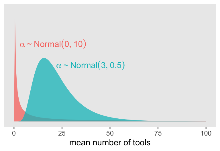

In this context, \(\alpha \sim \operatorname{Normal}(0, 10)\) has a very long tail on the outcome scale. The mean of the log-Normal distribution, recall, is \(\exp (\mu + \sigma^2/2)\). Here that is in code.

exp(0 + 10^2 / 2)

[1] 5.184706e+21

That is very large. Here’s the same thing in a simulation.

set.seed(11)

rnorm(1e4, 0, 10) |> 
  exp() |> 
  mean()

[1] 1.61276e+12

Now compute the mean for the other prior under consideration, \(\alpha \sim \operatorname{Normal}(3, 0.5)\).

exp(3 + 0.5^2 / 2)

[1] 22.7599

This is much smaller and more reasonable.

Now let’s prepare to make the top row of Figure 11.8. In this portion of the figure, we consider the implications of two competing priors for \(\beta\) while holding the prior for \(\alpha\) at \(\operatorname{Normal}(3, 0.5)\). The two \(\beta\) priors under consideration are \(\operatorname{Normal}(0, 10)\) and \(\operatorname{Normal}(0, 0.2)\).

set.seed(11)

# How many lines would you like?
n <- 100

# Simulate and wrangle
tibble(i = 1:n,
       a = rnorm(n, mean = 3, sd = 0.5)) |> 
  mutate(`beta%~%Normal(0*', '*10)`  = rnorm(n, mean = 0 , sd = 10),
         `beta%~%Normal(0*', '*0.2)` = rnorm(n, mean = 0 , sd = 0.2)) |> 
  pivot_longer(contains("beta"),
               values_to = "b",
               names_to = "prior") |> 
  expand_grid(x = seq(from = -2, to = 2, length.out = 100)) |> 
  mutate(prior = fct_rev(prior)) |> 
  
  # Plot
  ggplot(aes(x = x, y = exp(a + b * x), group = i)) +
  geom_line(alpha = 2/3, linewidth = 1/4) +
  labs(x = "log population (std)",
       y = "total tools") +
  coord_cartesian(ylim = c(0, 100)) +
  facet_wrap(~ prior, labeller = label_parsed)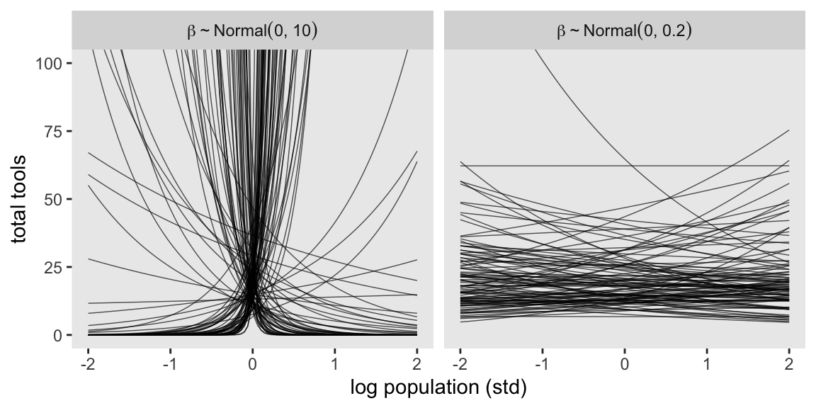

It turns out that many of the lines considered plausible under \(\operatorname{Normal}(0, 10)\) are disturbingly extreme. Here is what \(\alpha \sim \operatorname{Normal}(3, 0.5)\) and \(\beta \sim \operatorname{Normal}(0, 0.2)\) would mean when the \(x\)-axis is on the log population scale and the population scale.

set.seed(11)

prior <- tibble(
  i = 1:n,
  a = rnorm(n, mean = 3, sd = 0.5),
  b = rnorm(n, mean = 0, sd = 0.2)) |> 
  expand_grid(x = seq(from = log(100), to = log(200000), length.out = 100))

# Left
p1 <- prior |> 
  ggplot(aes(x = x, y = exp(a + b * x), group = i)) +
  geom_line(alpha = 2/3, linewidth = 1/4) +
  labs(x = "log population",
       y = "total tools") +
  coord_cartesian(xlim = c(log(100), log(200000)),
                  ylim = c(0, 500))
# Right
p2 <- prior |> 
  ggplot(aes(x = exp(x), y = exp(a + b * x), group = i)) +
  geom_line(alpha = 2/3, linewidth = 1/4) +
  scale_y_continuous(NULL, breaks = NULL) +
  xlab("population") +
  coord_cartesian(xlim = c(100, 200000),
                  ylim = c(0, 500))

# Combine, add facet strips, and display
(p1 | p2) &
  facet_wrap(~ "atop(alpha%~%Normal(3*', '*0.5), beta%~%Normal(0*', '*0.2))", 
             labeller = label_parsed)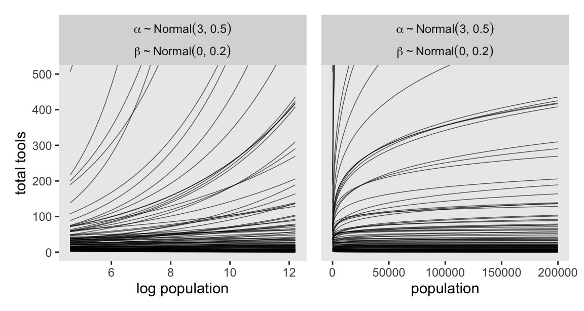

Okay, after settling on our two priors, the updated model formula is

\[ \begin{align*} y_i & \sim \operatorname{Poisson}(\lambda_i) \\ \log(\lambda_i) & = \alpha + \beta (x_i - \bar x) \\ \alpha & \sim \operatorname{Normal}(3, 0.5) \\ \beta & \sim \operatorname{Normal}(0, 0.2). \end{align*} \]

We’re finally ready to start fitting the models. First, define the stan_data.

stan_data <- d |> 
  select(total_tools, log_pop_std, cid) |> 
  compose_data()

# What?
str(stan_data)

List of 5
 $ total_tools: int [1:10(1d)] 13 22 24 43 33 19 40 28 55 71
 $ log_pop_std: num [1:10(1d)] -1.2915 -1.0886 -0.5158 -0.3288 -0.0443 ...
 $ cid        : num [1:10(1d)] 1 1 1 2 2 2 2 1 2 1
 $ n_cid      : int 2
 $ n          : int 10

Define model_code_11.9 and model_code_11.10.

# Intercept only
model_code_11.9 <- '
data {
  int<lower=1> n;
  array[n] int<lower=0> total_tools;
}
parameters {
  real a;  
}
model {
  total_tools ~ poisson(exp(a));
  a ~ normal(3, 0.5);
}
generated quantities {
  vector[n] log_lik;
  for (i in 1:n) log_lik[i] = poisson_lpmf(total_tools[i] | exp(a));
}
'

# Interaction model
model_code_11.10 <- '
data {
  int<lower=1> n;
  int<lower=1> n_cid;
  array[n] int cid;
  vector[n] log_pop_std;
  array[n] int<lower=0> total_tools;
}
parameters {
  vector[n_cid] a;
  vector[n_cid] b;
}
model {
  vector[n] lambda;
  lambda = exp(a[cid] + b[cid] .* log_pop_std);
  
  total_tools ~ poisson(lambda);
  a ~ normal(3, 0.5);
  b ~ normal(0, 0.2);
}
generated quantities {
  vector[n] log_lik;
  for (i in 1:n) log_lik[i] = poisson_lpmf(total_tools[i] | exp(a[cid[i]] + b[cid[i]] .* log_pop_std[i]));
}
'

As we discussed back in Section 1.3.3, we also could have fit these models with the poisson_log() function in place of poisson(), and computed the log_lik values with the poisson_log_lpmf() function in place of poisson_lpmf(). Those functions would have obviated our use of the exp() function for the linear model. Consider fitting the model both ways to see which is faster or returns better HMC diagnostics.

For now, we sample from the two posteriors as they’ve been currently defined with stan().

m11.9 <- stan(
  data = stan_data,
  model_code = model_code_11.9,
  cores = 4, seed = 11)

m11.10 <- stan(
  data = stan_data,
  model_code = model_code_11.10,
  cores = 4, seed = 11)

Compare the two models by the LOO.

l11.9 <- extract_log_lik(m11.9) |> loo()
l11.10 <- extract_log_lik(m11.10) |> loo()

Warning: Some Pareto k diagnostic values are too high. See help('pareto-k-diagnostic') for details.

loo_compare(l11.9, l11.10) |> 
  print(simplify = FALSE)

       elpd_diff se_diff elpd_loo se_elpd_loo p_loo se_p_loo looic se_looic
model2   0.0       0.0   -42.6      6.6         6.9   2.6     85.2  13.2   
model1 -28.1      16.4   -70.7     16.7         8.3   3.5    141.4  33.4

Like McElreath reported in the text, we have a Pareto-\(k\) warning. We can inspect the \(k\) values with loo::pareto_k_table().

pareto_k_table(l11.10)

Pareto k diagnostic values:
                         Count Pct.    Min. ESS
(-Inf, 0.7]   (good)     8     80.0%   344     
   (0.7, 1]   (bad)      1     10.0%   <NA>    
   (1, Inf)   (very bad) 1     10.0%   <NA>

Let’s take a closer look.

d |> 
  select(culture) |> 
  mutate(k = l11.10$diagnostics$pareto_k) |> 
  arrange(desc(k)) |> 
  mutate_if(is.double, round, digits = 2)

      culture    k
1      Hawaii 1.02
2       Tonga 0.83
3   Trobriand 0.56
4         Yap 0.55
5    Malekula 0.42
6       Manus 0.32
7     Tikopia 0.26
8    Lau Fiji 0.25
9  Santa Cruz 0.20
10      Chuuk 0.13

It turns out Hawaii is very influential. Figure 11.9 will clarify why. For a little practice while computing the trajectories, we’ll use an as_draws_df()-based workflow for the panel on the left, and use a spread_draws()-based workflow for the panel on the right.

# For subsetting the labels in the left panel
culture_vec <- c("Hawaii", "Tonga", "Trobriand", "Yap")

# Left
p1 <- as_draws_df(m11.10) |> 
  select(.draw, `a[1]`:`b[2]`) |> 
  pivot_longer(-.draw) |> 
  mutate(parameter = str_extract(name, "[a-z]"),
         cid = str_extract(name, "\\d")) |> 
  select(-name) |> 
  pivot_wider(names_from = parameter, values_from = value) |> 
  expand_grid(log_pop_std = seq(from = -4.5, to = 2.5, length.out = 100)) |> 
  mutate(total_tools = exp(a + b * log_pop_std)) |> 
  
  ggplot(aes(x = log_pop_std, y = total_tools,
             color = cid, fill = cid, group = cid)) +
  stat_lineribbon(.width = 0.89, alpha = 1/4) +
  geom_point(data = d |> 
               mutate(k = l11.10$diagnostics$pareto_k),
             aes(size = k)) +
  geom_text(data = d |> 
              mutate(k = l11.10$diagnostics$pareto_k) |> 
              mutate(label = str_c(culture, " (", round(k, digits = 2), ")"),
                     vjust = ifelse(total_tools > 30, -0.3, 1.3)) |> 
              filter(culture %in% culture_vec),
            aes(label = label, vjust = vjust),
            hjust = 1.1, size = 3) +
  labs(x = "log population (std)",
       y = "total tools") +
  coord_cartesian(xlim = range(d$log_pop_std),
                  ylim = c(0, 80))

# Right
p2 <- spread_draws(m11.10, a[cid], b[cid]) |> 
  mutate(cid = as.character(cid)) |> 
  expand_grid(log_pop_std = seq(from = -4.5, to = 2.5, length.out = 100)) |> 
  mutate(total_tools = exp(a + b * log_pop_std)) |>
  mutate(population = exp((log_pop_std * sd(log(d$population))) + mean(log(d$population)))) |> 
  
  ggplot(aes(x = population, y = total_tools,
             color = cid, fill = cid, group = cid)) +
  stat_lineribbon(.width = 0.89, alpha = 1/4) +
  geom_point(data = d |> 
               mutate(k = l11.10$diagnostics$pareto_k),
             aes(size = k)) +
  scale_x_continuous("population", breaks = c(0, 50000, 150000, 250000),
                     labels = scales::comma(c(0, 50000, 150000, 250000))) +
  scale_y_continuous(NULL, breaks = NULL) +
  coord_cartesian(xlim = range(d$population),
                  ylim = c(0, 80))

# Combine, adjust, and display
(p1 | p2) &
  scale_color_viridis_d(option = "A", end = 0.6) &
  scale_fill_viridis_d(option = "A", end = 0.6) &
  scale_size_continuous(range = c(0.1, 5), limits = c(0.1, 1.1)) &
  theme(legend.position = "none")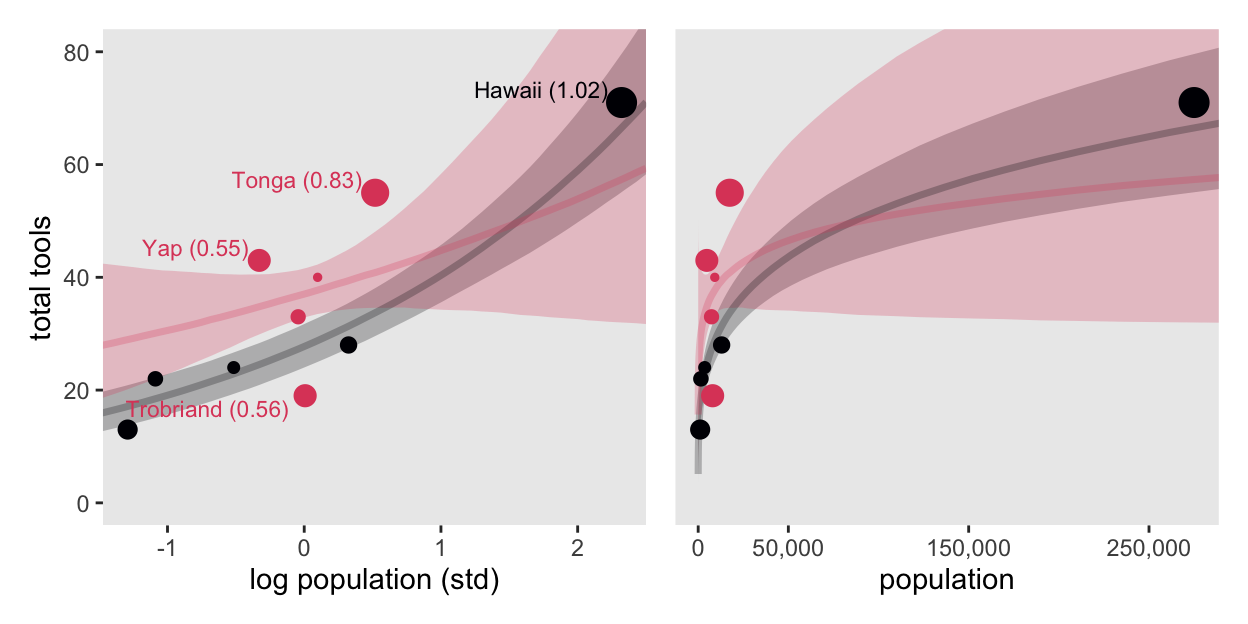

Hawaii is influential in that it has a very large population relative to the other islands.

11.2.1.1 Overthinking: Modeling tool innovation.

McElreath’s theoretical, or scientific, model for total_tools is

\[\widehat{\text{total-tools}} = \frac{\alpha_{\text{cid}[i]} \: \text{population}^{\beta_{\text{cid}[i]}}}{\gamma}.\]

We can use the Poisson likelihood to express this in a Bayesian model as

\[ \begin{align*} \text{total-tools} & \sim \operatorname{Poisson}(\lambda_i) \\ \lambda_i & = \left[ \exp (\alpha_{\text{cid}[i]}) \text{population}_i^{\beta_{\text{cid}[i]}} \right] / \gamma \\ \alpha_j & \sim \operatorname{Normal}(1, 1) \\ \beta_j & \sim \operatorname{Exponential}(1) \\ \gamma & \sim \operatorname{Exponential}(1), \end{align*} \]

where we exponentiate \(\alpha_{\text{cid}[i]}\) to restrict the posterior to zero and above. To fit that model with rstan, first we make some data d_pred for the predictions we’ll display in the plot.

d_pred <- tibble(
  population = seq(from = 0, to = 3e5, length.out = 101) |> 
    as.integer()) |> 
  expand_grid(cid = 1:2) |> 
  mutate(i = 1:n())

# What?
glimpse(d_pred)

Rows: 202
Columns: 3
$ population <int> 0, 0, 3000, 3000, 6000, 6000, 9000, 9000, 12000, 12000, 150…
$ cid        <int> 1, 2, 1, 2, 1, 2, 1, 2, 1, 2, 1, 2, 1, 2, 1, 2, 1, 2, 1, 2,…
$ i          <int> 1, 2, 3, 4, 5, 6, 7, 8, 9, 10, 11, 12, 13, 14, 15, 16, 17, …

Now make the stan_data.

stan_data <- d |> 
  mutate(population = as.double(population)) |>
  select(total_tools, population, cid) |>
  compose_data(population_pred = d_pred$population,
               cid_pred = d_pred$cid,
               n_pred = nrow(d_pred))

# What?
str(stan_data)

List of 8
 $ total_tools    : int [1:10(1d)] 13 22 24 43 33 19 40 28 55 71
 $ population     : num [1:10(1d)] 1100 1500 3600 4791 7400 ...
 $ cid            : num [1:10(1d)] 1 1 1 2 2 2 2 1 2 1
 $ n_cid          : int 2
 $ n              : int 10
 $ population_pred: int [1:202] 0 0 3000 3000 6000 6000 9000 9000 12000 12000 ...
 $ cid_pred       : int [1:202] 1 2 1 2 1 2 1 2 1 2 ...
 $ n_pred         : int 202

Define model_code_11.11.

model_code_11.11 <- '
data {
  int<lower=1> n;
  int<lower=1> n_cid;
  array[n] int cid;
  vector[n] population;
  array[n] int<lower=0> total_tools;
  // For predictions
  int<lower=1> n_pred;
  array[n_pred] int cid_pred;
  vector[n_pred] population_pred;
}
parameters {
  vector[n_cid] a;
  vector<lower=0>[n_cid] b;
  real<lower=0> g;
}
transformed parameters {
  vector[n] lambda;
  lambda = exp(a[cid]) .* population^b[cid] / g;
}
model {
  total_tools ~ poisson(lambda);
  a ~ normal(1, 1);
  b ~ exponential(1);
  g ~ exponential(1);
}
generated quantities {
  vector[n] log_lik;
  vector[n_pred] lambda_pred;
  
  for (i in 1:n) log_lik[i] = poisson_lpmf(total_tools[i] | lambda[i]);
  lambda_pred = exp(a[cid_pred]) .* population_pred^b[cid_pred] / g;
}
'

Sample from the posterior.

m11.11 <- stan(
  data = stan_data,
  model_code = model_code_11.11,
  cores = 4, seed = 11)

Check the model summary.

print(m11.11, pars = c("a", "b", "g"), probs = c(0.055, 0.945))

Inference for Stan model: anon_model.
4 chains, each with iter=2000; warmup=1000; thin=1; 
post-warmup draws per chain=1000, total post-warmup draws=4000.

     mean se_mean   sd  5.5% 94.5% n_eff Rhat
a[1] 0.92    0.02 0.68 -0.22  1.97  1383    1
a[2] 0.92    0.02 0.83 -0.42  2.26  1967    1
b[1] 0.26    0.00 0.03  0.20  0.32  1964    1
b[2] 0.29    0.00 0.11  0.12  0.46  1480    1
g    1.15    0.02 0.76  0.30  2.48  1605    1

Samples were drawn using NUTS(diag_e) at Thu Aug 15 11:44:42 2024.
For each parameter, n_eff is a crude measure of effective sample size,
and Rhat is the potential scale reduction factor on split chains (at 
convergence, Rhat=1).

Compute and check the PSIS-LOO estimates along with their diagnostic Pareto-\(k\) values.

l11.11 <- extract_log_lik(m11.11) |> loo()

Warning: Some Pareto k diagnostic values are too high. See help('pareto-k-diagnostic') for details.

print(l11.11)


Computed from 4000 by 10 log-likelihood matrix.

         Estimate   SE
elpd_loo    -40.6  6.0
p_loo         5.5  1.9
looic        81.3 12.0
------
MCSE of elpd_loo is NA.
MCSE and ESS estimates assume independent draws (r_eff=1).

Pareto k diagnostic values:
                         Count Pct.    Min. ESS
(-Inf, 0.7]   (good)     9     90.0%   274     
   (0.7, 1]   (bad)      1     10.0%   <NA>    
   (1, Inf)   (very bad) 0      0.0%   <NA>    
See help('pareto-k-diagnostic') for details.

We still have one high Pareto-\(k\) value. Recall that due to the very small sample size, this isn’t entirely surprising. If you’re curious, here’s a scatter plot of the Pareto-\(k\) values for this model and the last.

tibble(m11.10 = l11.10$diagnostics$pareto_k,
       m11.11 = l11.11$diagnostics$pareto_k) |> 
  
  ggplot(aes(x = m11.10, y = m11.11)) +
  geom_abline(color = "white") +
  geom_point() +
  scale_x_continuous(breaks = 0:5 / 5 + 0.1, limits = c(0.1, 1.1)) +
  scale_y_continuous(breaks = 0:5 / 5 + 0.1, limits = c(0.1, 1.1)) +
  labs(subtitle = expression(Pareto~italic(k)))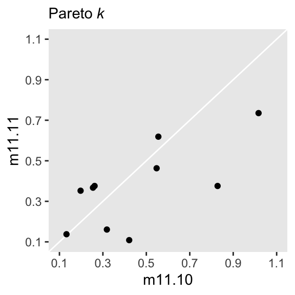

Okay, it’s time to make Figure 11.10. In the first line in the Wrangle section below, note how we’re using spread_draws() to extract the lambda_pred values we defined in the generated quantities, above.

# For the annotation
d_text <- distinct(d, cid, contact) |> 
  mutate(population  = c(210000, 72500),
         total_tools = c(59, 68),
         label       = str_c(contact, " contact"))

# Wrangle
spread_draws(m11.11, lambda_pred[i]) |> 
  left_join(d_pred, by = join_by(i)) |> 
  mutate(cid = as.character(cid)) |> 
  rename(total_tools = lambda_pred) |> 
  
  # Plot!
  ggplot(aes(x = population, y = total_tools,
             color = cid, fill = cid, group = cid)) +
  stat_lineribbon(.width = 0.89, alpha = 1/4) +
  geom_point(data = d |> 
               mutate(k = l11.11$diagnostics$pareto_k),
             aes(size = k)) +
  geom_text(data = d_text,
            aes(label = label)) +
  scale_x_continuous("population", breaks = c(0, 50000, 150000, 250000),
                     labels = scales::comma(c(0, 50000, 150000, 250000))) +
  scale_color_viridis_d(option = "A", end = 0.6) +
  scale_fill_viridis_d(option = "A", end = 0.6) +
  scale_size_continuous(range = c(0.1, 5), limits = c(0.1, 1)) +
  ylab("total tools") +
  coord_cartesian(xlim = range(d$population),
                  ylim = c(0, 80)) +
  theme(legend.position = "none")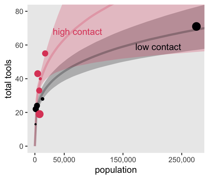

In case you were curious, here are the results if we compare m11.10 and m11.11 by the PSIS-LOO.

loo_compare(l11.10, l11.11) |> 
  print(simplify = FALSE)

       elpd_diff se_diff elpd_loo se_elpd_loo p_loo se_p_loo looic se_looic
model2   0.0       0.0   -40.6      6.0         5.5   1.9     81.3  12.0   
model1  -2.0       2.9   -42.6      6.6         6.9   2.6     85.2  13.2

11.2.2 Negative binomial (gamma-Poisson) models.

11.2.3 Example: Exposure and the offset.

Here we simulate our industrious monk data.

set.seed(11)

num_days <- 30
y        <- rpois(num_days, lambda = 1.5)

num_weeks <- 4
y_new     <- rpois(num_weeks, lambda = 0.5 * 7)

Now tidy the data and add log_days.

d <- tibble(
  y         = c(y, y_new), 
  days      = rep(c(1, 7), times = c(num_days, num_weeks)),  # this is the exposure
  monastery = rep(0:1, times = c(num_days, num_weeks))) |>
  mutate(log_days = log(days))

# What?
glimpse(d)

Rows: 34
Columns: 4
$ y         <int> 1, 0, 1, 0, 0, 4, 0, 1, 3, 0, 0, 1, 3, 3, 2, 2, 1, 1, 0, 1, …
$ days      <dbl> 1, 1, 1, 1, 1, 1, 1, 1, 1, 1, 1, 1, 1, 1, 1, 1, 1, 1, 1, 1, …
$ monastery <int> 0, 0, 0, 0, 0, 0, 0, 0, 0, 0, 0, 0, 0, 0, 0, 0, 0, 0, 0, 0, …
$ log_days  <dbl> 0, 0, 0, 0, 0, 0, 0, 0, 0, 0, 0, 0, 0, 0, 0, 0, 0, 0, 0, 0, …

Within the context of the Poisson likelihood, we can decompose \(\lambda\) into two parts, \(\mu\) (mean) and \(\tau\) (exposure), like this:

\[ y_i \sim \operatorname{Poisson}(\lambda_i) \\ \log \lambda_i = \log \frac{\mu_i}{\tau_i} = \log \mu_i - \log \tau_i. \]

Therefore, you can rewrite the equation if the exposure (\(\tau\)) varies in your data and you still want to model the mean (\(\mu\)). Using the model we’re about to fit as an example, here’s what that might look like:

\[ \begin{align*} y_i & \sim \operatorname{Poisson}(\mu_i) \\ \log \mu_i & = \color{blue}{\log \tau_i} + \alpha + \beta \text{monastery}_i \\ \alpha & \sim \operatorname{Normal}(0, 1) \\ \beta & \sim \operatorname{Normal}(0, 1), \end{align*} \]

where the offset \(\log \tau_i\) does not get a prior. In this context, its value is added directly to the right side of the formula. With the rstan package, we do this directly in the model block. First, though, let’s make the stan_data.

stan_data <- d |> 
  compose_data()

# What?
str(stan_data)

List of 5
 $ y        : int [1:34(1d)] 1 0 1 0 0 4 0 1 3 0 ...
 $ days     : num [1:34(1d)] 1 1 1 1 1 1 1 1 1 1 ...
 $ monastery: int [1:34(1d)] 0 0 0 0 0 0 0 0 0 0 ...
 $ log_days : num [1:34(1d)] 0 0 0 0 0 0 0 0 0 0 ...
 $ n        : int 34

Define model_code_11.12. Note how log_days does not get a coefficient in the lambda formula. It stands on its own.

model_code_11.12 <- '
data {
  int<lower=1> n;
  vector[n] log_days;
  vector[n] monastery;
  array[n] int<lower=0> y;
}
parameters {
  real a;
  real b;
}
model {
  y ~ poisson(exp(log_days + a + b * monastery));
  a ~ normal(0, 1);
  b ~ normal(0, 1);
}
'

Sample from the posterior.

m11.12 <- stan(
  data = stan_data,
  model_code = model_code_11.12,
  cores = 4, seed = 11)

As we look at the model summary, keep in mind that the parameters are on the per-one-unit-of-time scale. Since we simulated the data based on summary information from two units of time–one day and seven days–, this means the parameters are in the scale of \(\log (\lambda)\) per one day.

print(m11.12, probs = c(0.055, 0.945))

Inference for Stan model: anon_model.
4 chains, each with iter=2000; warmup=1000; thin=1; 
post-warmup draws per chain=1000, total post-warmup draws=4000.

       mean se_mean   sd   5.5%  94.5% n_eff Rhat
a     -0.01    0.00 0.18  -0.31   0.26  1776    1
b     -0.88    0.01 0.33  -1.40  -0.37  1861    1
lp__ -31.30    0.03 1.07 -33.31 -30.32  1639    1

Samples were drawn using NUTS(diag_e) at Thu Aug 15 11:46:33 2024.
For each parameter, n_eff is a crude measure of effective sample size,
and Rhat is the potential scale reduction factor on split chains (at 
convergence, Rhat=1).

To get the posterior distributions for average daily outputs for the old and new monasteries, respectively, we’ll use use the formulas

\[ \begin{align*} \lambda_\text{old} & = \exp (\alpha) \;\;\; \text{and} \\ \lambda_\text{new} & = \exp (\alpha + \beta_\text{monastery}). \end{align*} \]

Following those transformations, we’ll summarize the \(\lambda\) distributions with medians and 89% HDIs with help from the tidybayes::mean_hdi() function.

as_draws_df(m11.12) |>
  mutate(lambda_old = exp(a),
         lambda_new = exp(a + b)) |>
  pivot_longer(contains("lambda")) |> 
  mutate(name = factor(name, levels = c("lambda_old", "lambda_new"))) |>
  group_by(name) |>
  mean_hdi(value, .width = .89) |> 
  mutate_if(is.double, round, digits = 2)

# A tibble: 2 × 7
  name       value .lower .upper .width .point .interval
  <fct>      <dbl>  <dbl>  <dbl>  <dbl> <chr>  <chr>    
1 lambda_old  1      0.73   1.28   0.89 mean   hdi      
2 lambda_new  0.43   0.24   0.61   0.89 mean   hdi

Because we don’t know what seed McElreath used to simulate his data, our simulated data differed a little from his and, as a consequence, our results differ a little, too.

11.3 Multinomial and categorical models

11.3.1 Predictors matched to outcomes.

I will flesh this section out later.

11.3.2 Predictors matched to observations.

I will flesh this section out later.

11.3.2.1 Multinomial in disguise as Poisson.

Here we fit a multinomial likelihood by refactoring it to a series of Poisson models. Let’s retrieve the Berkeley data.

data(UCBadmit, package = "rethinking")
d <- UCBadmit
rm(UCBadmit)

Set up the stan_data.

stan_data <- d |> 
  # `reject` is a reserved word in Stan, and must not be used as variable name
  mutate(rej = reject) |> 
  select(admit, rej, applications) |> 
  compose_data()

# What?
str(stan_data)

List of 4
 $ admit       : int [1:12(1d)] 512 89 353 17 120 202 138 131 53 94 ...
 $ rej         : int [1:12(1d)] 313 19 207 8 205 391 279 244 138 299 ...
 $ applications: int [1:12(1d)] 825 108 560 25 325 593 417 375 191 393 ...
 $ n           : int 12

Define the model_code objects for the two complimentary models.

# Binomial model of overall admission probability
model_code_11.binom <- '
data {
  int<lower=1> n;
  array[n] int<lower=1> applications;
  array[n] int<lower=0> admit;
}
parameters {
  real a;
}
model {
  admit ~ binomial(applications, inv_logit(a));
  a ~ normal(0, 1.5);
}
'

# Poisson model of overall admission rate and rejection rate
model_code_11.pois <- '
data {
  int<lower=1> n;
  array[n] int<lower=1> applications;
  array[n] int<lower=0> admit;
  array[n] int<lower=0> rej;
}
parameters {
  real a1;
  real a2;
}
model {
  admit ~ poisson(exp(a1));
  rej ~ poisson(exp(a2));
  [a1, a2] ~ normal(0, 1.5);
}
'

Compile and extract the posterior draws for both with stan().

m11.binom <- stan(
  model_code = model_code_11.binom, 
  data = stan_data,
  chains = 3, cores = 3, seed = 11)

m11.pois <- stan(
  model_code = model_code_11.pois,
  data = stan_data,
  chains = 3, cores = 3, seed = 11)

Compare the two model summaries.

print(m11.binom, pars = "a", probs = c(0.055, 0.945))

Inference for Stan model: anon_model.
3 chains, each with iter=2000; warmup=1000; thin=1; 
post-warmup draws per chain=1000, total post-warmup draws=3000.

   mean se_mean   sd  5.5% 94.5% n_eff Rhat
a -0.46       0 0.03 -0.51 -0.41  1078    1

Samples were drawn using NUTS(diag_e) at Thu Aug 15 11:47:57 2024.
For each parameter, n_eff is a crude measure of effective sample size,
and Rhat is the potential scale reduction factor on split chains (at 
convergence, Rhat=1).

print(m11.pois, pars = c("a1", "a2"), probs = c(0.055, 0.945))

Inference for Stan model: anon_model.
3 chains, each with iter=2000; warmup=1000; thin=1; 
post-warmup draws per chain=1000, total post-warmup draws=3000.

   mean se_mean   sd 5.5% 94.5% n_eff Rhat
a1 4.98       0 0.02 4.94  5.02  2591    1
a2 5.44       0 0.02 5.41  5.47  3015    1

Samples were drawn using NUTS(diag_e) at Thu Aug 15 11:48:24 2024.
For each parameter, n_eff is a crude measure of effective sample size,
and Rhat is the potential scale reduction factor on split chains (at 
convergence, Rhat=1).

Though the model summaries look very different for the two models, they give the same answer, within MCMC simulation error, for the focal estimand \(p_\text{admit}\). We might explore that in a plot.

bind_rows(
  # Binomial
  as_draws_df(m11.binom) |> 
    transmute(p_admit = plogis(a)),
  # Poisson
  as_draws_df(m11.pois) |> 
    transmute(p_admit = exp(a1) / (exp(a1) + exp(a2)))
) |> 
  mutate(fit = rep(c("m11.binom", "m11.pois"), each = n() / 2)) |> 
  
  ggplot(aes(x = p_admit, y = fit)) +
  stat_halfeye(.width = 0.89) +
  scale_y_discrete(NULL, expand = expansion(mult = 0.1)) +
  xlab(expression(italic(p)[admit]))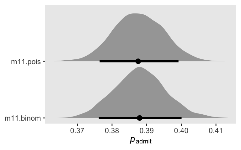

11.3.2.2 Overthinking: Multinomial-Poisson transformation.

11.4 Summary

Session info

sessionInfo()

R version 4.4.0 (2024-04-24)
Platform: aarch64-apple-darwin20
Running under: macOS Ventura 13.4

Matrix products: default
BLAS:   /Library/Frameworks/R.framework/Versions/4.4-arm64/Resources/lib/libRblas.0.dylib 
LAPACK: /Library/Frameworks/R.framework/Versions/4.4-arm64/Resources/lib/libRlapack.dylib;  LAPACK version 3.12.0

locale:
[1] en_US.UTF-8/en_US.UTF-8/en_US.UTF-8/C/en_US.UTF-8/en_US.UTF-8

time zone: America/Chicago
tzcode source: internal

attached base packages:
[1] stats     graphics  grDevices utils     datasets  methods   base     

other attached packages:
 [1] posterior_1.6.0    patchwork_1.2.0    loo_2.8.0          rstan_2.32.6      
 [5] StanHeaders_2.32.7 tidybayes_3.0.6    lubridate_1.9.3    forcats_1.0.0     
 [9] stringr_1.5.1      dplyr_1.1.4        purrr_1.0.2        readr_2.1.5       
[13] tidyr_1.3.1        tibble_3.2.1       ggplot2_3.5.1      tidyverse_2.0.0   

loaded via a namespace (and not attached):
 [1] gtable_0.3.5         tensorA_0.36.2.1     xfun_0.43           
 [4] QuickJSR_1.1.3       htmlwidgets_1.6.4    inline_0.3.19       
 [7] lattice_0.22-6       tzdb_0.4.0           vctrs_0.6.5         
[10] tools_4.4.0          generics_0.1.3       stats4_4.4.0        
[13] curl_5.2.1           parallel_4.4.0       fansi_1.0.6         
[16] pkgconfig_2.0.3      KernSmooth_2.23-22   Matrix_1.7-0        
[19] checkmate_2.3.1      distributional_0.4.0 RcppParallel_5.1.7  
[22] lifecycle_1.0.4      farver_2.1.1         compiler_4.4.0      
[25] munsell_0.5.1        codetools_0.2-20     htmltools_0.5.8.1   
[28] yaml_2.3.8           pillar_1.9.0         arrayhelpers_1.1-0  
[31] abind_1.4-5          tidyselect_1.2.1     digest_0.6.35       
[34] svUnit_1.0.6         stringi_1.8.4        labeling_0.4.3      
[37] fastmap_1.1.1        grid_4.4.0           colorspace_2.1-0    
[40] cli_3.6.3            magrittr_2.0.3       pkgbuild_1.4.4      
[43] utf8_1.2.4           withr_3.0.0          scales_1.3.0        
[46] backports_1.5.0      timechange_0.3.0     rmarkdown_2.26      
[49] matrixStats_1.3.0    gridExtra_2.3        hms_1.1.3           
[52] coda_0.19-4.1        evaluate_0.23        knitr_1.46          
[55] V8_4.4.2             ggdist_3.3.2         viridisLite_0.4.2   
[58] rlang_1.1.4          Rcpp_1.0.12          glue_1.7.0          
[61] rstudioapi_0.16.0    jsonlite_1.8.8       R6_2.5.1

11.1 Binomial regression

11.1.1 Logistic regression: Prosocial chimpanzees.

11.1.1.1 Overthinking: Adding log-probability calculations to a Stan model.

11.1.2 Relative shark and absolute deer.

11.1.2.1 Overthinking: Proportional odds and relative risk.

11.1.3 Aggregated binomial: Chimpanzees again, condensed.

11.1.4 Aggregated binomial: Graduate school admissions.

11.1.4.1 Rethinking: Simpson’s paradox is not a paradox.

11.2 Poisson regression

11.2.1 Example: Oceanic tool complexity.

11.2.1.1 Overthinking: Modeling tool innovation.

11.2.2 Negative binomial (gamma-Poisson) models.

11.2.3 Example: Exposure and the offset.

11.3 Multinomial and categorical models

11.3.1 Predictors matched to outcomes.

11.3.2 Predictors matched to observations.

11.3.2.1 Multinomial in disguise as Poisson.

11.3.2.2 Overthinking: Multinomial-Poisson transformation.

11.4 Summary

Session info

Comments