7  Examining the Multilevel Model’s Error Covariance Structure

In this chapter…, we focus on the model’s random effects as embodied in its error covariance structure. Doing so allows us to both describe the particular error covariance structure that the “standard” multilevel model for change invokes and it also allows us to broaden its representation to other—sometimes more tenable assumptions—about its behavior. (Singer & Willett, 2003, p. 243, emphasis in the original)

7.1 The “standard” specification of the multilevel model for change

Load the opposites_pp data (Willett, 1988).

library(tidyverse)

opposites_pp <- read_csv("~/Dropbox/Recoding Applied Longitudinal Data Analysis/data/opposites_pp.csv")

glimpse(opposites_pp)
Rows: 140
Columns: 6
$ id   <dbl> 1, 1, 1, 1, 2, 2, 2, 2, 3, 3, 3, 3, 4, 4, 4, 4, 5, 5, 5, 5, 6, 6, 6, 6, 7, 7, 7, 7, 8, 8, 8, 8, 9, 9, 9, 9, 10, 10,…
$ time <dbl> 0, 1, 2, 3, 0, 1, 2, 3, 0, 1, 2, 3, 0, 1, 2, 3, 0, 1, 2, 3, 0, 1, 2, 3, 0, 1, 2, 3, 0, 1, 2, 3, 0, 1, 2, 3, 0, 1, 2…
$ opp  <dbl> 205, 217, 268, 302, 219, 243, 279, 302, 142, 212, 250, 289, 206, 230, 248, 273, 190, 220, 229, 220, 165, 205, 207, …
$ cog  <dbl> 137, 137, 137, 137, 123, 123, 123, 123, 129, 129, 129, 129, 125, 125, 125, 125, 81, 81, 81, 81, 110, 110, 110, 110,…
$ ccog <dbl> 23.5429, 23.5429, 23.5429, 23.5429, 9.5429, 9.5429, 9.5429, 9.5429, 15.5429, 15.5429, 15.5429, 15.5429, 11.5429, 11…
$ wave <dbl> 1, 2, 3, 4, 1, 2, 3, 4, 1, 2, 3, 4, 1, 2, 3, 4, 1, 2, 3, 4, 1, 2, 3, 4, 1, 2, 3, 4, 1, 2, 3, 4, 1, 2, 3, 4, 1, 2, 3…

Willett (1988) clarified these data were simulated for pedagogical purposes, which will become important later on. For now, here’s our version of Table 7.1.

opposites_pp %>% 
  mutate(name = str_c("opp", wave)) %>% 
  select(id, name, opp, cog) %>% 
  
  pivot_wider(names_from = name, values_from = opp) %>% 
  select(id, starts_with("opp"), cog) %>% 
  head(n = 10)
# A tibble: 10 × 6
      id  opp1  opp2  opp3  opp4   cog
   <dbl> <dbl> <dbl> <dbl> <dbl> <dbl>
 1     1   205   217   268   302   137
 2     2   219   243   279   302   123
 3     3   142   212   250   289   129
 4     4   206   230   248   273   125
 5     5   190   220   229   220    81
 6     6   165   205   207   263   110
 7     7   170   182   214   268    99
 8     8    96   131   159   213   113
 9     9   138   156   197   200   104
10    10   216   252   274   298    96

The data are composed of 35 people’s scores on a cognitive task, across 4 time points.

opposites_pp %>% 
  count(id)
# A tibble: 35 × 2
      id     n
   <dbl> <int>
 1     1     4
 2     2     4
 3     3     4
 4     4     4
 5     5     4
 6     6     4
 7     7     4
 8     8     4
 9     9     4
10    10     4
# ℹ 25 more rows

Our first model will serve as a comparison model for all that follow. We’ll often refer to it as the standard multilevel model for change. You’ll see why in a bit. It follows the form

\[ \begin{align} \text{opp}_{ij} & = \pi_{0i} + \pi_{1i} \text{time}_{ij} + \epsilon_{ij}\\ \pi_{0i} & = \gamma_{00} + \gamma_{01} (\text{cog}_i - \overline{\text{cog}}) + \zeta_{0i}\\ \pi_{1i} & = \gamma_{10} + \gamma_{11} (\text{cog}_i - \overline{\text{cog}}) + \zeta_{1i} \\ \epsilon_{ij} & \stackrel{iid}{\sim} \operatorname{Normal}(0, \sigma_\epsilon) \\ \begin{bmatrix} \zeta_{0i} \\ \zeta_{1i} \end{bmatrix} & \stackrel{iid}{\sim} \operatorname{Normal} \left ( \begin{bmatrix} 0 \\ 0 \end{bmatrix}, \mathbf D \mathbf\Omega \mathbf D' \right ) \\ \mathbf D & = \begin{bmatrix} \sigma_0 & 0 \\ 0 & \sigma_1 \end{bmatrix} \\ \mathbf \Omega & = \begin{bmatrix} 1 & \rho_{01} \\ \rho_{01} & 1 \end{bmatrix}, \end{align} \]

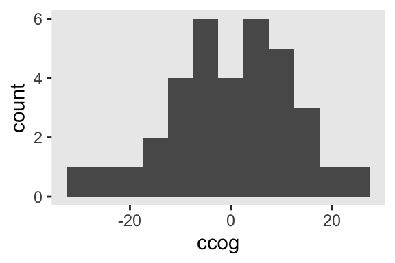
where the \((\text{cog}_i - \overline{\text{cog}})\) notation is meant to indicate we are mean centering the time-invariant covariate \(\text{cog}_i\). In the data, the mean-centered version is saved as ccog.

opposites_pp %>% 
  filter(wave == 1) %>% 
  
  ggplot(aes(ccog)) +
  geom_histogram(binwidth = 5) +
  theme(panel.grid = element_blank())

To keep things simple, we’ll be using brms default priors for all the models in this chapter. Fit the model.

library(brms)

fit7.1 <- brm(
  data = opposites_pp, 
  family = gaussian,
  opp ~ 0 + Intercept + time + ccog + time:ccog + (1 + time | id),
  iter = 2000, warmup = 1000, chains = 4, cores = 4,
  seed = 7,
  file = "fits/fit07.01")

Check the summary.

print(fit7.1, digits = 3)
 Family: gaussian 
  Links: mu = identity 
Formula: opp ~ 0 + Intercept + time + ccog + time:ccog + (1 + time | id) 
   Data: opposites_pp (Number of observations: 140) 
  Draws: 4 chains, each with iter = 2000; warmup = 1000; thin = 1;
         total post-warmup draws = 4000

Multilevel Hyperparameters:
~id (Number of levels: 35) 
                    Estimate Est.Error l-95% CI u-95% CI  Rhat Bulk_ESS Tail_ESS
sd(Intercept)         36.119     4.933   27.567   46.837 1.001     1249     1827
sd(time)              10.575     1.808    7.466   14.570 1.000     1289     2344
cor(Intercept,time)   -0.438     0.167   -0.711   -0.074 1.001     1501     2221

Regression Coefficients:
          Estimate Est.Error l-95% CI u-95% CI  Rhat Bulk_ESS Tail_ESS
Intercept  164.282     6.464  151.454  176.704 1.006      828     1301
time        26.962     2.093   22.917   31.209 1.003     1558     2290
ccog        -0.144     0.520   -1.179    0.888 1.004     1274     2011
time:ccog    0.439     0.170    0.104    0.770 1.001     1781     2433

Further Distributional Parameters:
      Estimate Est.Error l-95% CI u-95% CI  Rhat Bulk_ESS Tail_ESS
sigma   12.970     1.153   10.947   15.365 1.001     1727     2537

Draws were sampled using sampling(NUTS). For each parameter, Bulk_ESS
and Tail_ESS are effective sample size measures, and Rhat is the potential
scale reduction factor on split chains (at convergence, Rhat = 1).

If you’re curious, here’s the summary of our \(\sigma\) parameters transformed to the variance/covariance metric.

library(tidybayes)

levels <- c("sigma[epsilon]^2", "sigma[0]^2", "sigma[1]^2", "sigma[0][1]")

sigma <- as_draws_df(fit7.1) %>% 
  transmute(`sigma[0]^2` = sd_id__Intercept^2,
            `sigma[1]^2` = sd_id__time^2,
            `sigma[epsilon]^2` = sigma^2,
            `sigma[0][1]` = sd_id__Intercept * sd_id__time * cor_id__Intercept__time)

sigma %>% 
  pivot_longer(everything()) %>% 
  mutate(name = factor(name, levels = levels)) %>% 
  group_by(name) %>% 
  median_qi(value) %>% 
  mutate_if(is.double, round, digits = 2)
# A tibble: 4 × 7
  name             value .lower .upper .width .point .interval
  <fct>            <dbl>  <dbl>  <dbl>  <dbl> <chr>  <chr>    
1 sigma[epsilon]^2  166.  120.   236.    0.95 median qi       
2 sigma[0]^2       1274.  760.  2194.    0.95 median qi       
3 sigma[1]^2        109.   55.8  212.    0.95 median qi       
4 sigma[0][1]      -163. -394.   -22.4   0.95 median qi       

7.2 Using the composite model to understand assumptions about the error covariance matrix

Dropping the terms specifying the distributional assumptions, we can reexpress the model formula, from above, in the composite format as

\[ \begin{align} \text{opp}_{ij} & = [\gamma_{00} + \gamma_{10} \text{time}_{ij} + \gamma_{01} (\text{cog}_i - \overline{\text{cog}}) + \gamma_{11} (\text{cog}_i - \overline{\text{cog}}) \times \text{time}_{ij}] \\ & \;\;\; + [\zeta_{0i} + \zeta_{1i} \text{time}_{ij} + \epsilon_{ij}], \end{align} \]

where we’ve divided up the structural and stochastic components with our use of brackets. We might think of the terms of the stochastic portion as a composite residual, \(r_{ij} = [\epsilon_{ij} + \zeta_{0i} + \zeta_{1i} \text{time}_{ij}]\). Thus, we can rewrite the composite equation with the composite residual term \(r_{ij}\) as

\[ \text{opp}_{ij} = [\gamma_{00} + \gamma_{10} \text{time}_{ij} + \gamma_{01} (\text{cog}_i - \overline{\text{cog}}) + \gamma_{11} (\text{cog}_i - \overline{\text{cog}}) \times \text{time}_{ij}] + r_{ij}. \]

If we were willing to presume, as in OLS or single-level Bayesian regression, that all residuals are independent and normally distributed, we could express that in statistical notation as

\[\begin{align} \begin{bmatrix} r_{11} \\ r_{12} \\ r_{13} \\ r_{14} \\ r_{21} \\ r_{22} \\ r_{23} \\ r_{24} \\ \vdots \\ r_{n1} \\ r_{n2} \\ r_{n3} \\ r_{n4} \end{bmatrix} & \sim \mathcal{N} \begin{pmatrix} \begin{bmatrix} 0 \\ 0 \\ 0 \\ 0 \\ 0 \\ 0 \\ 0 \\ 0 \\ \vdots \\ 0 \\ 0 \\ 0 \\ 0 \\ \end{bmatrix}, \begin{bmatrix} \sigma_r^2 & 0 & 0 & 0 & 0 & 0 & 0 & 0 & \dots & 0 & 0 & 0 & 0 \\ 0 & \sigma_r^2 & 0 & 0 & 0 & 0 & 0 & 0 & \dots & 0 & 0 & 0 & 0 \\ 0 & 0 & \sigma_r^2 & 0 & 0 & 0 & 0 & 0 & \dots & 0 & 0 & 0 & 0 \\ 0 & 0 & 0 & \sigma_r^2 & 0 & 0 & 0 & 0 & \dots & 0 & 0 & 0 & 0 \\ 0 & 0 & 0 & 0 & \sigma_r^2 & 0 & 0 & 0 & \dots & 0 & 0 & 0 & 0 \\ 0 & 0 & 0 & 0 & 0 & \sigma_r^2 & 0 & 0 & \dots & 0 & 0 & 0 & 0 \\ 0 & 0 & 0 & 0 & 0 & 0 & \sigma_r^2 & 0 & \dots & 0 & 0 & 0 & 0 \\ 0 & 0 & 0 & 0 & 0 & 0 & 0 & \sigma_r^2 & \dots & 0 & 0 & 0 & 0 \\ \vdots & \vdots & \vdots & \vdots & \vdots & \vdots & \vdots & \vdots & \ddots & \vdots & \vdots & \vdots & \vdots & \\ 0 & 0 & 0 & 0 & 0 & 0 & 0 & 0 & \dots & \sigma_r^2 & 0 & 0 & 0 \\ 0 & 0 & 0 & 0 & 0 & 0 & 0 & 0 & \dots & 0 & \sigma_r^2 & 0 & 0 \\ 0 & 0 & 0 & 0 & 0 & 0 & 0 & 0 & \dots & 0 & 0 & \sigma_r^2 & 0 \\ 0 & 0 & 0 & 0 & 0 & 0 & 0 & 0 & \dots & 0 & 0 & 0 & \sigma_r^2 \end{bmatrix} \end{pmatrix}, \end{align}\]

where \(r_{ij}\) is the \(i\)th person’s residual on the \(j\)th time point. The variance/covariance matrix \(\mathbf \Sigma\) is diagonal (i.e., all the off-diagonal elements are 0’s) and homoscedastic (i.e., all the diagonal elements are the same value, \(\sigma_r^2\)).

These assumptions are absurd for longitudinal data, which is why we don’t analyze such data with single-level models. If we were to make the less restrictive assumptions that, within people, the residuals were correlated over time and were heteroscedastic, we could express that as

\[\begin{align} \begin{bmatrix} r_{11} \\ r_{12} \\ r_{13} \\ r_{14} \\ r_{21} \\ r_{22} \\ r_{23} \\ r_{24} \\ \vdots \\ r_{n1} \\ r_{n2} \\ r_{n3} \\ r_{n4} \end{bmatrix} & \sim \mathcal{N} \begin{pmatrix} \begin{bmatrix} 0 \\ 0 \\ 0 \\ 0 \\ 0 \\ 0 \\ 0 \\ 0 \\ \vdots \\ 0 \\ 0 \\ 0 \\ 0 \\ \end{bmatrix}, \begin{bmatrix} \sigma_{r_1}^2 & \sigma_{r_1 r_2} & \sigma_{r_1 r_3} & \sigma_{r_1 r_4} & 0 & 0 & 0 & 0 & \dots & 0 & 0 & 0 & 0 \\ \sigma_{r_2 r_1} & \sigma_{r_2}^2 & \sigma_{r_2 r_3} & \sigma_{r_2 r_4} & 0 & 0 & 0 & 0 & \dots & 0 & 0 & 0 & 0 \\ \sigma_{r_3 r_1} & \sigma_{r_3 r_2} & \sigma_{r_3}^2 & \sigma_{r_3 r_4} & 0 & 0 & 0 & 0 & \dots & 0 & 0 & 0 & 0 \\ \sigma_{r_4 r_1} & \sigma_{r_4 r_2} & \sigma_{r_4 r_3} & \sigma_{r_4}^2 & 0 & 0 & 0 & 0 & \dots & 0 & 0 & 0 & 0 \\ 0 & 0 & 0 & 0 & \sigma_{r_1}^2 & \sigma_{r_1 r_2} & \sigma_{r_1 r_3} & \sigma_{r_1 r_4} & \dots & 0 & 0 & 0 & 0 \\ 0 & 0 & 0 & 0 & \sigma_{r_2 r_1} & \sigma_{r_2}^2 & \sigma_{r_2 r_3} & \sigma_{r_2 r_4} & \dots & 0 & 0 & 0 & 0 \\ 0 & 0 & 0 & 0 & \sigma_{r_3 r_1} & \sigma_{r_3 r_2} & \sigma_{r_3}^2 & \sigma_{r_3 r_4} & \dots & 0 & 0 & 0 & 0 \\ 0 & 0 & 0 & 0 & \sigma_{r_4 r_1} & \sigma_{r_4 r_2} & \sigma_{r_4 r_3} & \sigma_{r_4}^2 & \dots & 0 & 0 & 0 & 0 \\ \vdots & \vdots & \vdots & \vdots & \vdots & \vdots & \vdots & \vdots & \ddots & \vdots & \vdots & \vdots & \vdots & \\ 0 & 0 & 0 & 0 & 0 & 0 & 0 & 0 & \dots & \sigma_{r_1}^2 & \sigma_{r_1 r_2} & \sigma_{r_1 r_3} & \sigma_{r_1 r_4} \\ 0 & 0 & 0 & 0 & 0 & 0 & 0 & 0 & \dots & \sigma_{r_2 r_1} & \sigma_{r_2}^2 & \sigma_{r_2 r_3} & \sigma_{r_2 r_4} \\ 0 & 0 & 0 & 0 & 0 & 0 & 0 & 0 & \dots & \sigma_{r_3 r_1} & \sigma_{r_3 r_2} & \sigma_{r_3}^2 & \sigma_{r_3 r_4} \\ 0 & 0 & 0 & 0 & 0 & 0 & 0 & 0 & \dots & \sigma_{r_4 r_1} & \sigma_{r_4 r_2} & \sigma_{r_4 r_3} & \sigma_{r_4}^2 \end{bmatrix} \end{pmatrix}. \end{align}\]

this kind of structure can be called block diagonal, which means the off-diagonal elements are zero between persons, but allowed to be non-zero within persons (i.e., within blocks). The zero elements between person blocks explicate how the residuals are independent between persons. Notice that the variances on the diagonal vary across the four time points (i.e., \(\sigma_{r_1}^2, \dots, \sigma_{r_4}^2\)). Yet also notice that the block for one person is identical to the block for all others. Thus, this model allows for heterogeneity across time within persons, but homogeneity between persons.

We can express this in the more compact notation,

\[\begin{align} r & \sim \mathcal{N} \begin{pmatrix} \mathbf 0, \begin{bmatrix} \mathbf{\Sigma}_r & \mathbf 0 & \mathbf 0 & \dots & \mathbf 0 \\ \mathbf 0 & \mathbf{\Sigma}_r & \mathbf 0 & \dots & \mathbf 0 \\ \mathbf 0 & \mathbf 0 & \mathbf{\Sigma}_r & \dots & \mathbf 0 \\ \vdots & \vdots & \vdots & \ddots & \mathbf 0 \\ \mathbf 0 & \mathbf 0 & \mathbf 0 & \mathbf 0 & \mathbf{\Sigma}_r \end{bmatrix} \end{pmatrix}, \;\;\; \text{where} \\ \mathbf{\Sigma}_r & = \begin{bmatrix} \sigma_{r_1}^2 & \sigma_{r_1 r_2} & \sigma_{r_1 r_3} & \sigma_{r_1 r_4} \\ \sigma_{r_2 r_1} & \sigma_{r_2}^2 & \sigma_{r_2 r_3} & \sigma_{r_2 r_4} \\ \sigma_{r_3 r_1} & \sigma_{r_3 r_2} & \sigma_{r_3}^2 & \sigma_{r_3 r_4} \\ \sigma_{r_4 r_1} & \sigma_{r_4 r_2} & \sigma_{r_4 r_3} & \sigma_{r_4}^2 \end{bmatrix}. \end{align}\]

The bulk of the rest of the material in this chapter will focus around how different models handle \(\mathbf{\Sigma}_r\). The standard multilevel growth model has one way. There are many others.

7.2.1 Variance of the composite residual

Under the conventional multilevel growth model

\[ \begin{align} \sigma_{r_j}^2 & = \operatorname{Var} \left ( \epsilon_{ij} + \zeta_{0i} + \zeta_{1i} \text{time}_j \right ) \\ & = \sigma_\epsilon^2 + \sigma_0^2 + 2 \sigma_{01} \text{time}_j + \sigma_1^2 \text{time}_j^2. \end{align} \]

Here’s how to use our posterior samples to compute \(\sigma_{r_1}^2, \dots, \sigma_{r_4}^2\).

sigma %>% 
  mutate(iter = 1:n()) %>% 
  expand(nesting(iter, `sigma[epsilon]^2`, `sigma[0]^2`, `sigma[1]^2`, `sigma[0][1]`),
         time = 0:3) %>% 
  mutate(r = `sigma[epsilon]^2` + `sigma[0]^2` + 2 * `sigma[0][1]` * time + `sigma[1]^2` * time^2) %>% 
  mutate(name = str_c("sigma[italic(r)[", time + 1, "]]^2")) %>% 
  
  ggplot(aes(x = r, y = name)) +
  stat_halfeye(.width = 0.95, size = 1) +
  scale_x_continuous("marginal posterior", expand = expansion(mult = c(0, 0.05)), limits = c(0, NA)) +
  scale_y_discrete(NULL, labels = ggplot2:::parse_safe) +
  coord_cartesian(ylim = c(1.5, 4.2)) +
  theme(panel.grid = element_blank())

As is often the case with variance parameters, the posteriors show marked right skew. Here are the numeric summaries.

sigma %>% 
  mutate(iter = 1:n()) %>% 
  expand(nesting(iter, `sigma[epsilon]^2`, `sigma[0]^2`, `sigma[1]^2`, `sigma[0][1]`),
         time = 0:3) %>% 
  mutate(r = `sigma[epsilon]^2` + `sigma[0]^2` + 2 * `sigma[0][1]` * time + `sigma[1]^2` * time^2) %>% 
  mutate(name = str_c("sigma[italic(r)[", time + 1, "]]^2")) %>% 
  group_by(name) %>% 
  median_qi(r)
# A tibble: 4 × 7
  name                      r .lower .upper .width .point .interval
  <chr>                 <dbl>  <dbl>  <dbl>  <dbl> <chr>  <chr>    
1 sigma[italic(r)[1]]^2 1443.   929.  2365.   0.95 median qi       
2 sigma[italic(r)[2]]^2 1219.   811.  1979.   0.95 median qi       
3 sigma[italic(r)[3]]^2 1209.   813.  1995.   0.95 median qi       
4 sigma[italic(r)[4]]^2 1421.   915.  2431.   0.95 median qi       

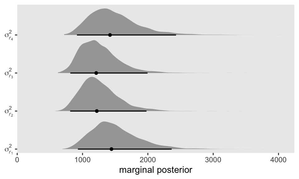
Though our precise numeric values are different from those in the text, we see the same overall pattern. Using our posterior medians, we can update \(\mathbf{\Sigma}_r\) to

\[ \begin{align} \hat{\mathbf{\Sigma}}_r & = \begin{bmatrix} 1430 & \hat{\sigma}_{r_1 r_2} & \hat{\sigma}_{r_1 r_3} & \hat{\sigma}_{r_1 r_4} \\ \hat{\sigma}_{r_2 r_1} & 1201 & \hat{\sigma}_{r_2 r_3} & \hat{\sigma}_{r_2 r_4} \\ \hat{\sigma}_{r_3 r_1} & \hat{\sigma}_{r_3 r_2} & 1203 & \hat{\sigma}_{r_3 r_4} \\ \hat{\sigma}_{r_4 r_1} & \hat{\sigma}_{r_4 r_2} & \hat{\sigma}_{r_4 r_3} & 1416 \end{bmatrix}. \end{align} \]

For the opposites-naming data, composite residual variance is greatest at the beginning and end of data collection and smaller in between. And, while not outrageously heteroscedastic, this situation is clearly beyond the bland homoscedasticity that we routinely assume for residuals in cross-sectional data. (p. 252)

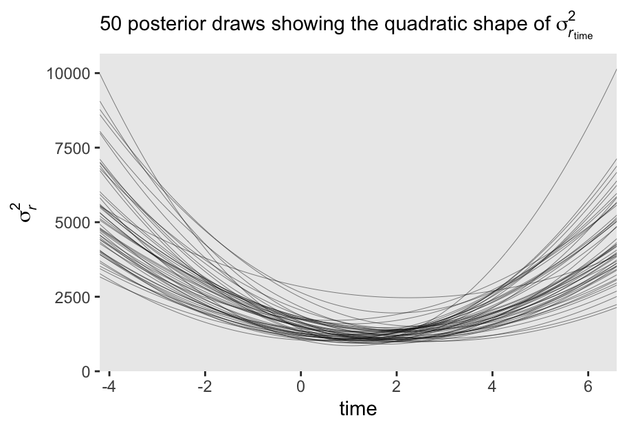
If you work through the equation at the beginning of this section–which I am not going to do, here–, you’ll see that the standard multilevel growth model is set up such that the residual variance follows a quadratic function with time. To give a sense, here we plot the expected \(\sigma_r^2\) values over a wider and more continuous range of time values.

set.seed(7)

sigma %>% 
  mutate(iter = 1:n()) %>% 
  slice_sample(n = 50) %>% 
  expand(nesting(iter, `sigma[epsilon]^2`, `sigma[0]^2`, `sigma[1]^2`, `sigma[0][1]`),
         time = seq(from = -4.2, to = 6.6, length.out = 200)) %>% 
  mutate(r = `sigma[epsilon]^2` + `sigma[0]^2` + 2 * `sigma[0][1]` * time + `sigma[1]^2` * time^2) %>% 
  
  ggplot(aes(x = time, y = r, group = iter)) +
  geom_line(linewidth = 1/6, alpha = 1/2) +
  scale_x_continuous(expand = c(0, 0)) +
  scale_y_continuous(expression(sigma[italic(r)]^2),
                     expand = expansion(mult = c(0, 0.05)), limits = c(0, NA)) +
  labs(subtitle = expression("50 posterior draws showing the quadratic shape of "*sigma[italic(r)[time]]^2)) +
  theme(panel.grid = element_blank())

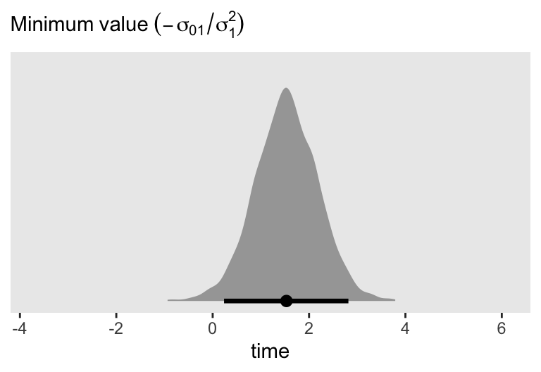
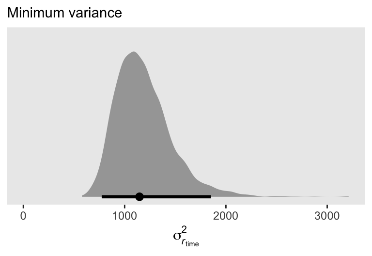
Since we have 4,000 posterior draws for all the parameters, we also have 4,000 posterior draws for the quadratic curve. Here we just show 50. The curve is at its minimum at \(\text{time} = -(\sigma_{01} / \sigma_1^2)\). Since we have posterior distributions for \(\sigma_{01}\) and \(\sigma_1^2\), we’ll also have a posterior distribution for the minimum point. Here it is.

sigma %>% 
  mutate(minimum = -`sigma[0][1]` / `sigma[1]^2`) %>% 
  
  ggplot(aes(x = minimum)) +
  stat_halfeye(.width = 0.95) +
  scale_x_continuous("time", expand = c(0, 0), limits = c(-4.2, 6.6)) +
  scale_y_continuous(NULL, breaks = NULL) +
  labs(subtitle = expression(Minimum~value~(-sigma[0][1]/sigma[1]^2))) +
  theme(panel.grid = element_blank())

If we plug those minimum time values into the equation for \(\sigma_{r_\text{time}}^2\), we’ll get the posterior distribution for the minimum variance value.

sigma %>% 
  mutate(minimum = -`sigma[0][1]` / `sigma[1]^2`) %>% 
  mutate(r = `sigma[epsilon]^2` + `sigma[0]^2` + 2 * `sigma[0][1]` * minimum + `sigma[1]^2` * minimum^2) %>% 
  
  ggplot(aes(x = r)) +
  stat_halfeye(.width = 0.95) +
  scale_x_continuous(expression(sigma[italic(r)[time]]^2), limits = c(0, NA)) +
  scale_y_continuous(NULL, breaks = NULL) +
  labs(subtitle = "Minimum variance") +
  theme(panel.grid = element_blank())

Here’s the numeric summary.

sigma %>% 
  mutate(minimum = -`sigma[0][1]` / `sigma[1]^2`) %>% 
  mutate(r = `sigma[epsilon]^2` + `sigma[0]^2` + 2 * `sigma[0][1]` * minimum + `sigma[1]^2` * minimum^2) %>% 
  median_qi(r)
# A tibble: 1 × 6
      r .lower .upper .width .point .interval
  <dbl>  <dbl>  <dbl>  <dbl> <chr>  <chr>    
1 1147.   773.  1853.   0.95 median qi       

7.2.2 Covariance of the composite residuals

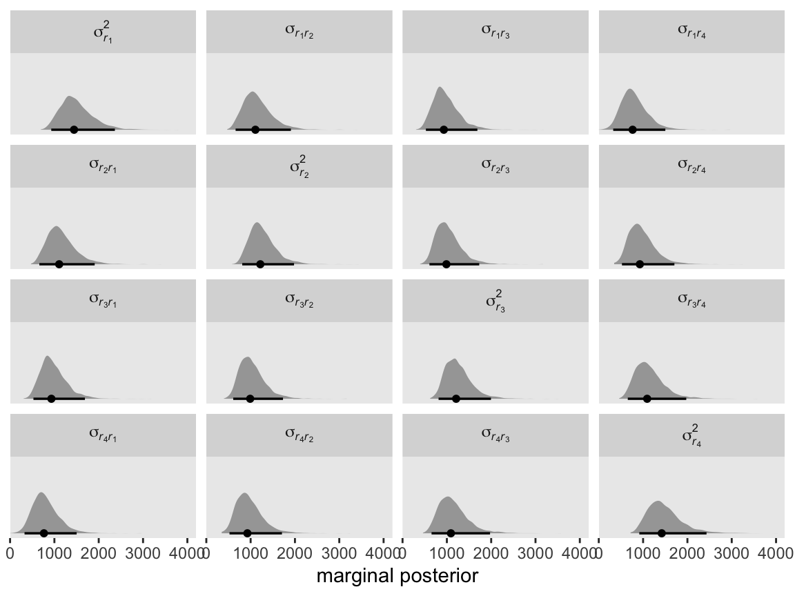
In addition to the variances in \(\mathbf{\Sigma}_r\), we might focus on the off-diagonal covariances, too. We can define the covariance between two time points \(\sigma_{r_j, r_{j'}}\) as

\[ \sigma_{r_j, r_{j'}} = \sigma_0^2 + \sigma_{01} (t_j + t_{j'}) + \sigma_1^2 t_j t_{j'}, \]

where \(\sigma_0^2\), \(\sigma_{01}\) and \(\sigma_1^2\) all have their usual interpretation, and \(t_j\) and \(t_{j'}\) are the numeric values for whatever variable is used to index time in the model, which is time in the case of fit7.1. Here we compute and plot the marginal posteriors for all \(4 \times 4 = 16\) parameters.

# arrange the panels
levels <- c(
  "sigma[italic(r)[1]]^2", "sigma[italic(r)[1]][italic(r)[2]]", "sigma[italic(r)[1]][italic(r)[3]]", "sigma[italic(r)[1]][italic(r)[4]]", 
  "sigma[italic(r)[2]][italic(r)[1]]", "sigma[italic(r)[2]]^2", "sigma[italic(r)[2]][italic(r)[3]]", "sigma[italic(r)[2]][italic(r)[4]]", 
  "sigma[italic(r)[3]][italic(r)[1]]", "sigma[italic(r)[3]][italic(r)[2]]", "sigma[italic(r)[3]]^2", "sigma[italic(r)[3]][italic(r)[4]]", 
  "sigma[italic(r)[4]][italic(r)[1]]", "sigma[italic(r)[4]][italic(r)[2]]", "sigma[italic(r)[4]][italic(r)[3]]", "sigma[italic(r)[4]]^2")

# wrangle
sigma <- sigma %>% 
  mutate(
    `sigma[italic(r)[1]]^2` = `sigma[epsilon]^2` + `sigma[0]^2` + 2 * `sigma[0][1]` * 0 + `sigma[1]^2` * 0^2,
    `sigma[italic(r)[2]]^2` = `sigma[epsilon]^2` + `sigma[0]^2` + 2 * `sigma[0][1]` * 1 + `sigma[1]^2` * 1^2,
    `sigma[italic(r)[3]]^2` = `sigma[epsilon]^2` + `sigma[0]^2` + 2 * `sigma[0][1]` * 2 + `sigma[1]^2` * 2^2,
    `sigma[italic(r)[4]]^2` = `sigma[epsilon]^2` + `sigma[0]^2` + 2 * `sigma[0][1]` * 3 + `sigma[1]^2` * 3^2,
    
    `sigma[italic(r)[2]][italic(r)[1]]` = `sigma[0]^2` + `sigma[0][1]` * (1 + 0) + `sigma[1]^2` * 1 * 0,
    `sigma[italic(r)[3]][italic(r)[1]]` = `sigma[0]^2` + `sigma[0][1]` * (2 + 0) + `sigma[1]^2` * 2 * 0,
    `sigma[italic(r)[4]][italic(r)[1]]` = `sigma[0]^2` + `sigma[0][1]` * (3 + 0) + `sigma[1]^2` * 3 * 0,
    `sigma[italic(r)[3]][italic(r)[2]]` = `sigma[0]^2` + `sigma[0][1]` * (2 + 1) + `sigma[1]^2` * 2 * 1,
    `sigma[italic(r)[4]][italic(r)[2]]` = `sigma[0]^2` + `sigma[0][1]` * (3 + 1) + `sigma[1]^2` * 3 * 1,
    `sigma[italic(r)[4]][italic(r)[3]]` = `sigma[0]^2` + `sigma[0][1]` * (3 + 2) + `sigma[1]^2` * 3 * 2,
    
    `sigma[italic(r)[1]][italic(r)[2]]` = `sigma[0]^2` + `sigma[0][1]` * (0 + 1) + `sigma[1]^2` * 0 * 1,
    `sigma[italic(r)[1]][italic(r)[3]]` = `sigma[0]^2` + `sigma[0][1]` * (0 + 2) + `sigma[1]^2` * 0 * 2,
    `sigma[italic(r)[2]][italic(r)[3]]` = `sigma[0]^2` + `sigma[0][1]` * (1 + 2) + `sigma[1]^2` * 1 * 2,
    `sigma[italic(r)[1]][italic(r)[4]]` = `sigma[0]^2` + `sigma[0][1]` * (0 + 3) + `sigma[1]^2` * 0 * 3,
    `sigma[italic(r)[2]][italic(r)[4]]` = `sigma[0]^2` + `sigma[0][1]` * (1 + 3) + `sigma[1]^2` * 1 * 3,
    `sigma[italic(r)[3]][italic(r)[4]]` = `sigma[0]^2` + `sigma[0][1]` * (2 + 3) + `sigma[1]^2` * 2 * 3)

sigma %>% 
  select(contains("italic")) %>% 
  pivot_longer(everything()) %>%  
  mutate(name = factor(name, levels = levels)) %>% 
  
  # plot!
  ggplot(aes(x = value)) +
  stat_halfeye(.width = 0.95, size = 1) +
  scale_x_continuous("marginal posterior", expand = expansion(mult = c(0, 0.05))) +
  scale_y_discrete(NULL, breaks = NULL) +
  coord_cartesian(xlim = c(0, 4000),
                  ylim = c(0.5, NA)) +
  theme(panel.grid = element_blank()) +
  facet_wrap(~ name, labeller = label_parsed)

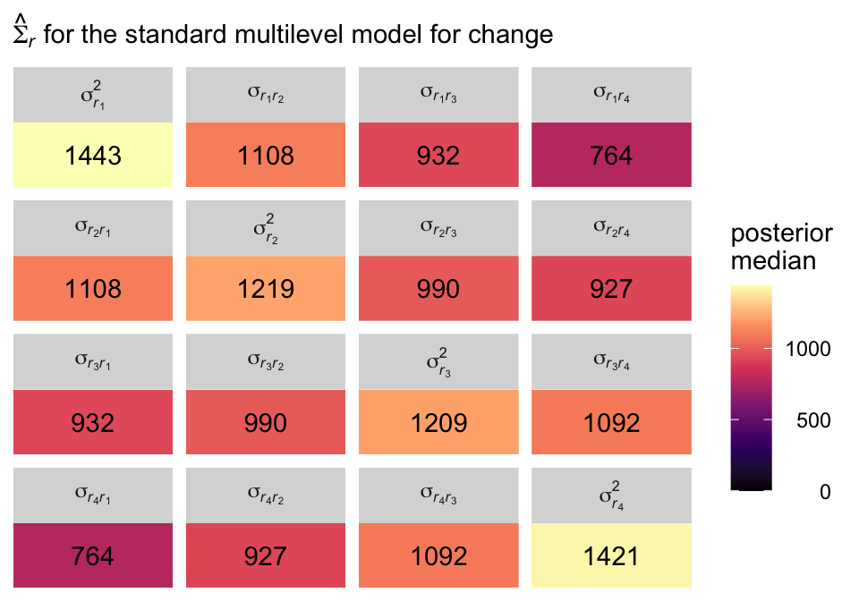
It might be helpful to reduce the complexity of this plot by focusing on the posterior medians. With a little help from geom_tile() and geom_text(), we’ll make a plot version of the matrix at the top of page 255 in the text.

sigma %>% 
  select(contains("italic")) %>% 
  pivot_longer(everything()) %>%  
  mutate(name = factor(name, levels = levels)) %>% 
  group_by(name) %>% 
  median_qi(value) %>% 
  mutate(label = round(value, digits = 0)) %>% 
  
  ggplot(aes(x = 0, y = 0)) +
  geom_tile(aes(fill = value)) +
  geom_text(aes(label = label)) +
  scale_fill_viridis_c("posterior\nmedian", option = "A", limits = c(0, NA)) +
  scale_x_continuous(NULL, breaks = NULL, expand = c(0, 0)) +
  scale_y_continuous(NULL, breaks = NULL, expand = c(0, 0)) +
  labs(subtitle = expression(hat(Sigma)[italic(r)]*" for the standard multilevel model for change")) +
  theme(legend.text = element_text(hjust = 1)) +
  facet_wrap(~ name, labeller = label_parsed)

Although our posterior median values differ a bit from the REML values reported in the text, the overall pattern holds. Hopefully the coloring in the plot helps highlight what Singer and Willett described as a “‘band diagonal’ structure, in which the overall magnitude of the residual covariances tends to decline in diagonal ‘bands’ the further you get from the main diagonal” (p. 255).

One of the consequences for this structure is that in cases where both \(\sigma_1^2 \rightarrow 0\) and \(\sigma_{01} \rightarrow 0\), the residual covariance matrix becomes compound symmetric, which is:

\[ \begin{align} \mathbf{\Sigma}_r & = \begin{bmatrix} \sigma_\epsilon^2 + \sigma_0^2 & \sigma_0^2 & \sigma_0^2 & \sigma_0^2 \\ \sigma_0^2 & \sigma_\epsilon^2 + \sigma_0^2 & \sigma_0^2 & \sigma_0^2 \\ \sigma_0^2 & \sigma_0^2 & \sigma_\epsilon^2 + \sigma_0^2 & \sigma_0^2 \\ \sigma_0^2 & \sigma_0^2 & \sigma_0^2 & \sigma_\epsilon^2 + \sigma_0^2 \end{bmatrix}. \end{align} \]

Compound symmetric error covariance structures are particularly common in longitudinal data, especially if the slopes of the change trajectories do not differ much asroc people. Regardless of these special cases, however, the most sensible question to ask of your data is whether the error covariance structure that the “standard” multilevel model for change demands is realistic when applied to data in practice? The answer to this question will determine whether the standard model can be applied ubiquitously, as question we soon address. (pp. 255–256)

7.2.3 Autocorrelation of the composite residuals

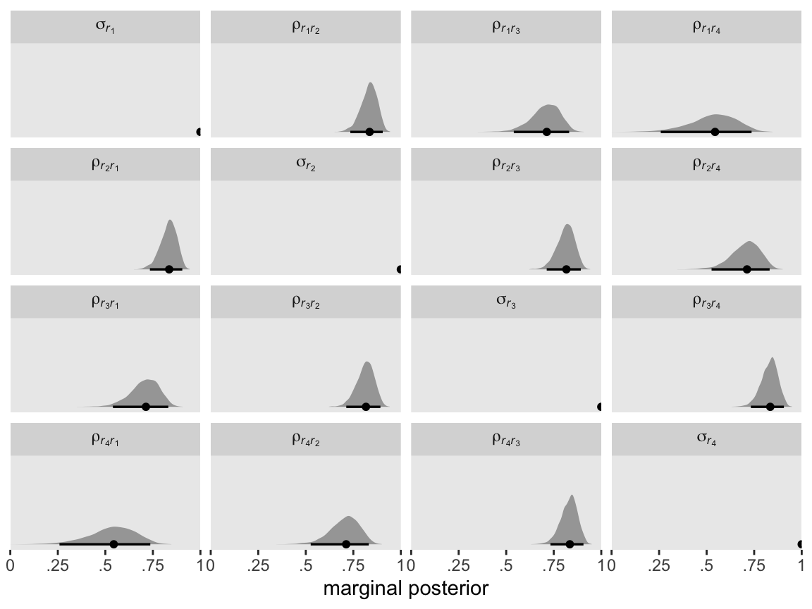
We can use the following equation to convert our \(\mathbf{\Sigma}_r\) into a correlation matrix:

\[\rho_{r_j r_{j^\prime}} = \sigma_{r_j r_{j^\prime}} \Big / \sqrt{\sigma_{r_j}^2 \sigma_{r_{j^\prime}}^2}.\]

Here we use the formula and plot the posteriors.

# arrange the panels
levels <- c(
  "sigma[italic(r)[1]]", "rho[italic(r)[1]][italic(r)[2]]", "rho[italic(r)[1]][italic(r)[3]]", "rho[italic(r)[1]][italic(r)[4]]", 
  "rho[italic(r)[2]][italic(r)[1]]", "sigma[italic(r)[2]]", "rho[italic(r)[2]][italic(r)[3]]", "rho[italic(r)[2]][italic(r)[4]]", 
  "rho[italic(r)[3]][italic(r)[1]]", "rho[italic(r)[3]][italic(r)[2]]", "sigma[italic(r)[3]]", "rho[italic(r)[3]][italic(r)[4]]", 
  "rho[italic(r)[4]][italic(r)[1]]", "rho[italic(r)[4]][italic(r)[2]]", "rho[italic(r)[4]][italic(r)[3]]", "sigma[italic(r)[4]]")

sigma <- sigma %>% 
  select(contains("italic")) %>% 
  mutate(
    `sigma[italic(r)[1]]` = `sigma[italic(r)[1]]^2` / sqrt(`sigma[italic(r)[1]]^2`^2),
    `rho[italic(r)[2]][italic(r)[1]]` = `sigma[italic(r)[2]][italic(r)[1]]` / sqrt(`sigma[italic(r)[2]]^2` * `sigma[italic(r)[1]]^2`),
    `rho[italic(r)[3]][italic(r)[1]]` = `sigma[italic(r)[3]][italic(r)[1]]` / sqrt(`sigma[italic(r)[3]]^2` * `sigma[italic(r)[1]]^2`),
    `rho[italic(r)[4]][italic(r)[1]]` = `sigma[italic(r)[4]][italic(r)[1]]` / sqrt(`sigma[italic(r)[4]]^2` * `sigma[italic(r)[1]]^2`),
    
    `rho[italic(r)[1]][italic(r)[2]]` = `sigma[italic(r)[1]][italic(r)[2]]` / sqrt(`sigma[italic(r)[1]]^2` * `sigma[italic(r)[2]]^2`),
    `sigma[italic(r)[2]]` = `sigma[italic(r)[2]]^2` / sqrt(`sigma[italic(r)[2]]^2`^2),
    `rho[italic(r)[3]][italic(r)[2]]` = `sigma[italic(r)[3]][italic(r)[2]]` / sqrt(`sigma[italic(r)[3]]^2` * `sigma[italic(r)[2]]^2`),
    `rho[italic(r)[4]][italic(r)[2]]` = `sigma[italic(r)[4]][italic(r)[2]]` / sqrt(`sigma[italic(r)[4]]^2` * `sigma[italic(r)[2]]^2`),
    
    `rho[italic(r)[1]][italic(r)[3]]` = `sigma[italic(r)[1]][italic(r)[3]]` / sqrt(`sigma[italic(r)[1]]^2` * `sigma[italic(r)[3]]^2`),
    `rho[italic(r)[2]][italic(r)[3]]` = `sigma[italic(r)[2]][italic(r)[3]]` / sqrt(`sigma[italic(r)[2]]^2` * `sigma[italic(r)[3]]^2`),
    `sigma[italic(r)[3]]` = `sigma[italic(r)[3]]^2` / sqrt(`sigma[italic(r)[3]]^2`^2),
    `rho[italic(r)[4]][italic(r)[3]]` = `sigma[italic(r)[4]][italic(r)[3]]` / sqrt(`sigma[italic(r)[4]]^2` * `sigma[italic(r)[3]]^2`),
    
    `rho[italic(r)[1]][italic(r)[4]]` = `sigma[italic(r)[1]][italic(r)[4]]` / sqrt(`sigma[italic(r)[1]]^2` * `sigma[italic(r)[4]]^2`),
    `rho[italic(r)[2]][italic(r)[4]]` = `sigma[italic(r)[2]][italic(r)[4]]` / sqrt(`sigma[italic(r)[2]]^2` * `sigma[italic(r)[4]]^2`),
    `rho[italic(r)[3]][italic(r)[4]]` = `sigma[italic(r)[3]][italic(r)[4]]` / sqrt(`sigma[italic(r)[3]]^2` * `sigma[italic(r)[4]]^2`),
    `sigma[italic(r)[4]]` = `sigma[italic(r)[4]]^2` / sqrt(`sigma[italic(r)[4]]^2`^2))

sigma %>% 
  select(`sigma[italic(r)[1]]`:`sigma[italic(r)[4]]`) %>% 
  pivot_longer(everything()) %>%  
  mutate(name = factor(name, levels = levels)) %>% 
  
  # plot!
  ggplot(aes(x = value)) +
  stat_halfeye(.width = 0.95, size = 1) +
  scale_x_continuous("marginal posterior", expand = c(0, 0),
                     breaks = 0:4 / 4, labels = c("0", ".25", ".5", ".75", "1")) +
  scale_y_discrete(NULL, breaks = NULL) +
  coord_cartesian(xlim = c(0, 1),
                  ylim = c(0.5, NA)) +
  theme(panel.grid = element_blank()) +
  facet_wrap(~ name, labeller = label_parsed)

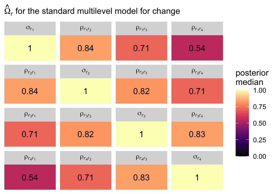
As before, it might be helpful to reduce the complexity of this plot by focusing on the posterior medians. We’ll make a plot version of the correlation matrix in the middle of page 256 in the text.

sigma %>% 
  select(`sigma[italic(r)[1]]`:`sigma[italic(r)[4]]`) %>% 
  pivot_longer(everything()) %>%  
  mutate(name = factor(name, levels = levels)) %>% 
  group_by(name) %>% 
  median_qi(value) %>% 
  mutate(label = round(value, digits = 2)) %>% 
  
  ggplot(aes(x = 0, y = 0)) +
  geom_tile(aes(fill = value)) +
  geom_text(aes(label = label)) +
  scale_fill_viridis_c("posterior\nmedian", option = "A", limits = c(0, 1)) +
  scale_x_continuous(NULL, breaks = NULL, expand = c(0, 0)) +
  scale_y_continuous(NULL, breaks = NULL, expand = c(0, 0)) +
  labs(subtitle = expression(hat(Omega)[italic(r)]*" for the standard multilevel model for change")) +
  theme(legend.text = element_text(hjust = 1)) +
  facet_wrap(~ name, labeller = label_parsed)

The correlation matrix has an even more pronounced band-diagonal structure. Thus even though the standard multilevel model of change does not contain an explicit autocorrelation parameter \(\rho\), the model does account for residual autocorrelation. We might take this even further. Notice the parameters \(\rho_{r_2, r_1}\), \(\rho_{r_3, r_2}\), and \(\rho_{r_4, r_3}\) are all autocorrelations of the first order, and further note how similar their posterior medians all are. Here’s a summary of the average of those three parameters, which we’ll just call \(\rho\).

sigma %>% 
  # take the average of the three parameters
  transmute(rho = (`rho[italic(r)[2]][italic(r)[1]]` + `rho[italic(r)[3]][italic(r)[2]]` + `rho[italic(r)[4]][italic(r)[3]]`) / 3) %>% 
  # summarize
  median_qi()
# A tibble: 1 × 6
    rho .lower .upper .width .point .interval
  <dbl>  <dbl>  <dbl>  <dbl> <chr>  <chr>    
1 0.828  0.740  0.897   0.95 median qi       

If you look at the “estimate” column in Table 7.3 (pp. 258–259), you’ll see the \(\hat \rho\) values for the autoregressive and heterogeneous-autoregressive models are very similar to the \(\hat \rho\) posterior we just computed for the standard multilevel model of change. The standard multilevel model of change accounts for autocorrelation, but it does so without an explicit \(\rho\) parameter.

7.3 Postulating an alternative error covariance structure

Singer and Willett wrote:

it is easy to specify alternative covariance structures for the composite residual and determine analytically which specification—the “standard” or an alternative—fits best. You already possess the analytic tools and skills needed for this work. (p. 257)

Frequentest R users would likely do this with the nlme package (Pinheiro et al., 2021). Recent additions to brms makes this largely possible, but not completely so. The six error structures listed in this section were:

  • unstructured,
  • compound symmetric,
  • heterogeneous compound symmetric,
  • autoregressive,
  • heterogeneous autoregressive, and
  • Toeplitz.

The Toeplitz structure is not currently available with brms, but we can experiment with the first five. For details, see issue #403 in the brms GitHub repo.

7.3.1 Unstructured error covariance matrix

Models using an unstructured error covariance matrix include \(k (k + 1) / 2\) variance/covariance parameters, where \(k\) is the number of time waves in the data. In the case of our opposites_pp data, we can compute the number of parameters as follows.

k <- 4
k * (k + 1) / 2
[1] 10

We end up with 4 variances and 6 covariances. Following the notation Singer and Willett used in the upper left corner of Table 7.3 (p. 258), we can express this as

\[ \begin{align} \mathbf{\Sigma}_r & = \begin{bmatrix} \sigma_1^2 & \sigma_{12} & \sigma_{13} & \sigma_{14} \\ \sigma_{21} & \sigma_2^2 & \sigma_{23} & \sigma_{24} \\ \sigma_{31} & \sigma_{32} & \sigma_3^2 & \sigma_{34} \\ \sigma_{41} & \sigma_{42} & \sigma_{43} & \sigma_4^2 \end{bmatrix}. \end{align} \]

The great appeal of an unstructured error covariance structure is that it places no restrictions on the structure of \(\mathbf{\Sigma}_r\). For a given set of fixed effects, its deviance statistic will always be the smallest of any error covariance structure. If you have just a few waves of data, this choice can be attractive. But if you have many waves, it can require an exorbitant number of parameters… [However,] the “standard” model requires only 3 variance components (\(\sigma_0^2\), \(\sigma_1^2\), and \(\sigma_\epsilon^2\)) and one covariance component, \(\sigma_{01}\). (p. 260)

To fit the unstructured model with brms, we use the unstr() function. Notice how we’ve dropped the usual (1 + time | id) syntax. Instead, we indicate the data are temporally structured by the time variable by setting time = time within unstr(), and we indicate the data are grouped by id by setting gr = id, also within unstr(). Also, notice we’ve wrapped the entire model formula within the bf() function. The second line within the bf() function has sigma on the left side of the ~ operator, which is something we haven’t seen before. With that line, we have allowed the residual variance \(\sigma_\epsilon\) to vary across time points. By default, brms will use the log link, to insure the model for \(\sigma_{\epsilon j}\) will never predict negative variances.

fit7.2 <- brm(
  data = opposites_pp, 
  family = gaussian,
  bf(opp ~ 0 + Intercept + time + ccog + time:ccog + unstr(time = time, gr = id),
     sigma ~ 0 + factor(time)),
  iter = 2000, warmup = 1000, chains = 4, cores = 4,
  seed = 7,
  file = "fits/fit07.02")

Check the summary.

print(fit7.2, digits = 3, robust = T)
 Family: gaussian 
  Links: mu = identity; sigma = log 
Formula: opp ~ 0 + Intercept + time + ccog + time:ccog + unstr(time = time, gr = id) 
         sigma ~ 0 + factor(time)
   Data: opposites_pp (Number of observations: 140) 
  Draws: 4 chains, each with iter = 2000; warmup = 1000; thin = 1;
         total post-warmup draws = 4000

Correlation Structures:
             Estimate Est.Error l-95% CI u-95% CI  Rhat Bulk_ESS Tail_ESS
cortime(0,1)    0.751     0.070    0.583    0.862 1.000     2317     2772
cortime(0,2)    0.659     0.088    0.441    0.801 1.000     2152     2910
cortime(1,2)    0.807     0.058    0.652    0.897 1.001     2525     2717
cortime(0,3)    0.336     0.140    0.033    0.576 1.001     2290     2824
cortime(1,3)    0.637     0.098    0.408    0.787 1.001     3011     3144
cortime(2,3)    0.735     0.076    0.540    0.848 1.000     2963     3200

Regression Coefficients:
                  Estimate Est.Error l-95% CI u-95% CI  Rhat Bulk_ESS Tail_ESS
Intercept          165.505     5.751  154.795  177.194 1.001     3098     3063
time                26.613     2.018   22.366   30.716 1.000     3125     3018
ccog                -0.109     0.462   -1.005    0.810 1.000     3444     2960
time:ccog            0.456     0.163    0.135    0.802 1.000     3233     2746
sigma_factortime0    3.571     0.117    3.357    3.824 1.002     2587     2530
sigma_factortime1    3.458     0.113    3.253    3.688 1.001     2123     2406
sigma_factortime2    3.496     0.106    3.294    3.724 1.002     2196     2410
sigma_factortime3    3.519     0.114    3.313    3.753 1.000     2817     2771

Draws were sampled using sampling(NUTS). For each parameter, Bulk_ESS
and Tail_ESS are effective sample size measures, and Rhat is the potential
scale reduction factor on split chains (at convergence, Rhat = 1).

There’s a lot of exciting things going on in that output. We’ll start with the bottom 4 rows in the Population-Level Effects section, which contains our the summaries for our \(\log (\sigma_{\epsilon j})\) parameters. To get them out of the log metric, we exponentiate. Here’s a quick conversion.

fixef(fit7.2)[5:8, -2] %>% exp()
                  Estimate     Q2.5    Q97.5
sigma_factortime0 35.73391 28.71447 45.80566
sigma_factortime1 31.88199 25.87892 39.96905
sigma_factortime2 33.09534 26.93729 41.44291
sigma_factortime3 33.87613 27.47317 42.65918

Now let’s address the new Correlation Structures section of the print() output. Just as brms decomposes the typical multilevel model level-2 variance/covariance matrix \(\mathbf{\Sigma}\) as

\[ \begin{align} \mathbf \Sigma & = \mathbf D \mathbf \Omega \mathbf D, \text{where} \\ \mathbf D & = \begin{bmatrix} \sigma_0 & 0 \\ 0 & \sigma_1 \end{bmatrix} \text{and} \\ \mathbf \Omega & = \begin{bmatrix} 1 & \rho \\ \rho & 1 \end{bmatrix}, \end{align} \]

the same kind of thing happens when we fit a model with an unstructured variance/covariance matrix with the unstr() function. The print() output returned posterior summaries for the elements of the correlation matrix \(\mathbf \Omega\) in the Correlation Structures section, and it returned posterior summaries for the elements of the diagonal matrix of standard deviations \(\mathbf D\) in the last four rows of the Population-Level Effects section. But notice that instead of \(2 \times 2\) matrices like we got with our conventional growth model fit7.1, both \(\mathbf D\) and \(\mathbf \Omega\) are now \(4 \times 4\) matrices right out of the gate. Thus if we use the posterior medians from the print() output as our point estimates, we can express the \(\hat{\mathbf \Sigma}\) matrix from our unstructured fit7.2 model as

\[ \begin{align} \mathbf \Sigma & = \mathbf D \mathbf \Omega \mathbf D \\ \hat{\mathbf D} & = \begin{bmatrix} 35.6 & 0 & 0 & 0 \\ 0 & 31.6 & 0 & 0 \\ 0 & 0 & 33.0 & 0 \\ 0 & 0 & 0 & 33.7 \end{bmatrix} \\ \hat{\mathbf \Omega} & = \begin{bmatrix} 1 & .75 & .66 & .33 \\ .75 & 1 & .81 & .64 \\ .66 & .81 & 1 & .73 \\ .33 & .64 & .73 & 1 \end{bmatrix}. \end{align} \]

Here’s how to compute and summarize the \(\mathbf D\) and \(\mathbf \Omega\) parameters with the as_draws_df() output.

# wrangle
sigma.us <- as_draws_df(fit7.2) %>%
  transmute(`sigma[1]` = exp(b_sigma_factortime0),
            `sigma[2]` = exp(b_sigma_factortime1),
            `sigma[3]` = exp(b_sigma_factortime2),
            `sigma[4]` = exp(b_sigma_factortime3),
            
            `rho[12]` = cortime__0__1,
            `rho[13]` = cortime__0__2,
            `rho[14]` = cortime__0__3,
            `rho[23]` = cortime__1__2,
            `rho[24]` = cortime__1__3,
            `rho[34]` = cortime__2__3,
            
            `rho[21]` = cortime__0__1, 
            `rho[31]` = cortime__0__2, 
            `rho[32]` = cortime__1__2, 
            `rho[41]` = cortime__0__3, 
            `rho[42]` = cortime__1__3, 
            `rho[43]` = cortime__2__3)

# summarize
sigma.us %>% 
  pivot_longer(everything()) %>% 
  group_by(name) %>% 
  median_qi(value) %>% 
  mutate_if(is.double, round, digits = 2)
# A tibble: 16 × 7
   name     value .lower .upper .width .point .interval
   <chr>    <dbl>  <dbl>  <dbl>  <dbl> <chr>  <chr>    
 1 rho[12]   0.75   0.58   0.86   0.95 median qi       
 2 rho[13]   0.66   0.44   0.8    0.95 median qi       
 3 rho[14]   0.34   0.03   0.58   0.95 median qi       
 4 rho[21]   0.75   0.58   0.86   0.95 median qi       
 5 rho[23]   0.81   0.65   0.9    0.95 median qi       
 6 rho[24]   0.64   0.41   0.79   0.95 median qi       
 7 rho[31]   0.66   0.44   0.8    0.95 median qi       
 8 rho[32]   0.81   0.65   0.9    0.95 median qi       
 9 rho[34]   0.73   0.54   0.85   0.95 median qi       
10 rho[41]   0.34   0.03   0.58   0.95 median qi       
11 rho[42]   0.64   0.41   0.79   0.95 median qi       
12 rho[43]   0.73   0.54   0.85   0.95 median qi       
13 sigma[1] 35.6   28.7   45.8    0.95 median qi       
14 sigma[2] 31.8   25.9   40.0    0.95 median qi       
15 sigma[3] 33.0   26.9   41.4    0.95 median qi       
16 sigma[4] 33.8   27.5   42.7    0.95 median qi       

Since Singer and Willett preferred the variance/covariance parameterization for \(\mathbf \Sigma\), we’ll practice wrangling the posterior draws to transform our results into that metric, too.

# transform
sigma.us <- sigma.us %>% 
  transmute(`sigma[1]^2` = `sigma[1]`^2,
            `sigma[12]` = `sigma[1]` * `sigma[2]` * `rho[12]`,
            `sigma[13]` = `sigma[1]` * `sigma[3]` * `rho[13]`,
            `sigma[14]` = `sigma[1]` * `sigma[4]` * `rho[14]`,
            
            `sigma[21]` = `sigma[2]` * `sigma[1]` * `rho[21]`,
            `sigma[2]^2` = `sigma[2]`^2,
            `sigma[23]` = `sigma[2]` * `sigma[3]` * `rho[23]`,
            `sigma[24]` = `sigma[2]` * `sigma[4]` * `rho[24]`,
            
            `sigma[31]` = `sigma[3]` * `sigma[1]` * `rho[31]`,
            `sigma[32]` = `sigma[3]` * `sigma[2]` * `rho[32]`,
            `sigma[3]^2` = `sigma[3]`^2,
            `sigma[34]` = `sigma[3]` * `sigma[4]` * `rho[34]`,
            
            `sigma[41]` = `sigma[4]` * `sigma[1]` * `rho[41]`,
            `sigma[42]` = `sigma[4]` * `sigma[2]` * `rho[42]`,
            `sigma[43]` = `sigma[4]` * `sigma[3]` * `rho[43]`,
            `sigma[4]^2` = `sigma[4]`^2)

# summarize
sigma.us %>% 
  pivot_longer(everything()) %>% 
  group_by(name) %>% 
  median_qi(value) %>% 
  mutate_if(is.double, round, digits = 2)
# A tibble: 16 × 7
   name       value .lower .upper .width .point .interval
   <chr>      <dbl>  <dbl>  <dbl>  <dbl> <chr>  <chr>    
 1 sigma[1]^2 1264.  825.   2098.   0.95 median qi       
 2 sigma[12]   840.  503.   1438.   0.95 median qi       
 3 sigma[13]   765.  429.   1321.   0.95 median qi       
 4 sigma[14]   393.   40.5   846.   0.95 median qi       
 5 sigma[2]^2 1008.  670.   1598.   0.95 median qi       
 6 sigma[21]   840.  503.   1438.   0.95 median qi       
 7 sigma[23]   841.  520.   1390.   0.95 median qi       
 8 sigma[24]   677.  367.   1176.   0.95 median qi       
 9 sigma[3]^2 1087.  726.   1718.   0.95 median qi       
10 sigma[31]   765.  429.   1321.   0.95 median qi       
11 sigma[32]   841.  520.   1390.   0.95 median qi       
12 sigma[34]   806.  484.   1375.   0.95 median qi       
13 sigma[4]^2 1139.  755.   1820.   0.95 median qi       
14 sigma[41]   393.   40.5   846.   0.95 median qi       
15 sigma[42]   677.  367.   1176.   0.95 median qi       
16 sigma[43]   806.  484.   1375.   0.95 median qi       

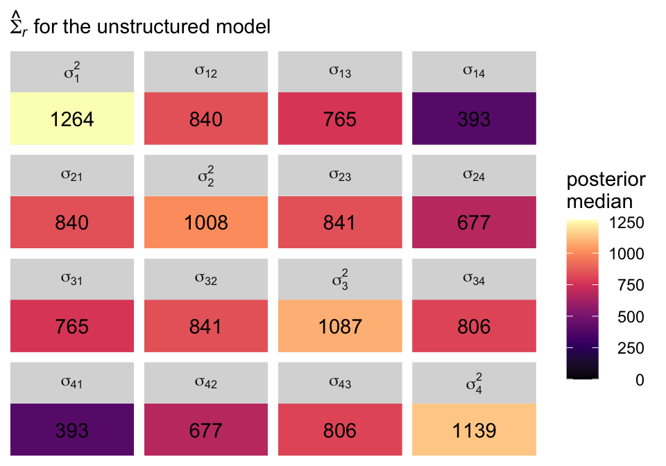
But again, I suspect it will be easier to appreciate our posterior \(\hat{\mathbf \Sigma}\) in a tile plot. Here’s a summary using the posterior medians, similar to what Singer and Willett reported in the rightmost column of Table 7.3.

levels <- c(
  "sigma[1]^2", "sigma[12]", "sigma[13]", "sigma[14]", 
  "sigma[21]", "sigma[2]^2", "sigma[23]", "sigma[24]", 
  "sigma[31]", "sigma[32]", "sigma[3]^2", "sigma[34]", 
  "sigma[41]", "sigma[42]", "sigma[43]", "sigma[4]^2")

sigma.us %>% 
  pivot_longer(everything()) %>%  
  mutate(name = factor(name, levels = levels)) %>% 
  group_by(name) %>% 
  median_qi(value) %>% 
  mutate(label = round(value, digits = 0)) %>% 
  
  ggplot(aes(x = 0, y = 0)) +
  geom_tile(aes(fill = value)) +
  geom_text(aes(label = label, color = value < 1),
            show.legend = F) +
  scale_fill_viridis_c("posterior\nmedian", option = "A", limits = c(0, NA)) +
  scale_color_manual(values = c("black", "white")) +
  scale_x_continuous(NULL, breaks = NULL, expand = c(0, 0)) +
  scale_y_continuous(NULL, breaks = NULL, expand = c(0, 0)) +
  labs(subtitle = expression(hat(Sigma)[italic(r)]*" for the unstructured model")) +
  theme(legend.text = element_text(hjust = 1)) +
  facet_wrap(~ name, labeller = label_parsed)

In case you’re curious, here’s the variance/covariance matrix from the sample data.

fit7.2$data %>% 
  select(id, time, opp) %>% 
  pivot_wider(names_from = time, values_from = opp) %>% 
  select(-id) %>% 
  cov() %>% 
  round(digits = 0)
     0    1    2    3
0 1309  976  922  563
1  976 1125 1021  855
2  922 1021 1292 1081
3  563  855 1081 1415

The brms default priors are weakly regularizing, particularly the LKJ prior for the correlation matrix \(\mathbf \Omega\), and I believe this is why the values from our model are systemically lower that the sample statistics. If you find this upsetting, collect more data, which hill help the likelihood dominate the prior.

7.3.2 Compound symmetric error covariance matrix

“A compound symmetric error covariance matrix requires just two parameters, labeled \(\sigma^2\) and \(\sigma_1^2\) in table 7.3” (p. 260). From the table, we see that matrix follows the form

\[ \begin{align} \mathbf{\Sigma}_r & = \begin{bmatrix} \sigma^2 + \sigma_1^2 & \sigma_1^2 & \sigma_1^2 & \sigma_1^2 \\ \sigma_1^2 & \sigma^2 + \sigma_1^2 & \sigma_1^2 & \sigma_1^2 \\ \sigma_1^2 & \sigma_1^2 & \sigma^2 + \sigma_1^2 & \sigma_1^2 \\ \sigma_1^2 & \sigma_1^2 & \sigma_1^2 & \sigma^2 + \sigma_1^2 \end{bmatrix}, \end{align} \]

where \(\sigma_1^2\) does not have the same meaning we’ve become accustomed to (i.e., the level-2 variance in linear change over time). The meaning of \(\sigma^2\) might also be a little opaque. Happily, there’s another way to express this matrix, which is a modification of the heterogeneous compound symmetric matrix we see listed in Table 7.3. That alternative is:

\[ \begin{align} \mathbf{\Sigma}_r & = \begin{bmatrix} \sigma_\epsilon^2 & \sigma_\epsilon^2 \rho & \sigma_\epsilon^2 \rho & \sigma_\epsilon^2 \rho \\ \sigma_\epsilon^2 \rho & \sigma_\epsilon^2 & \sigma_\epsilon^2 \rho & \sigma_\epsilon^2 \rho \\ \sigma_\epsilon^2 \rho & \sigma_\epsilon^2 \rho & \sigma_\epsilon^2 & \sigma_\epsilon^2 \rho \\ \sigma_\epsilon^2 \rho & \sigma_\epsilon^2 \rho & \sigma_\epsilon^2 \rho & \sigma_\epsilon^2 \end{bmatrix}, \end{align} \]

where the term on the diagonal, \(\sigma_\epsilon^2\), is the residual variance, which is constrained to equality across all four time points. In all cells in the off-diagonal, we see \(\sigma_\epsilon^2\) multiplied by \(\rho\). In this parameterization, \(\rho\) is the correlation between time points, and that correlation is constrained to equality across all possible pairs of time points. Although this notation is a little different from the notation used in the text, I believe it will help us interpret our model. As we’ll see, brms uses this alternative parameterization.

To fit the compound symmetric model with brms, we use the cosy() function. Notice how like with the unstructured model fit7.2, we’ve dropped the usual (1 + time | id) syntax. Instead, we impose compound symmetry within persons by setting gr = id within cosy().

fit7.3 <- brm(
  data = opposites_pp,
  family = gaussian,
  opp ~ 0 + Intercept + time + ccog + time:ccog + cosy(gr = id),
  iter = 2000, warmup = 1000, chains = 4, cores = 4,
  seed = 7,
  file = "fits/fit07.03")

Check the model summary.

print(fit7.3, digits = 3)
 Family: gaussian 
  Links: mu = identity 
Formula: opp ~ 0 + Intercept + time + ccog + time:ccog + cosy(gr = id) 
   Data: opposites_pp (Number of observations: 140) 
  Draws: 4 chains, each with iter = 2000; warmup = 1000; thin = 1;
         total post-warmup draws = 4000

Correlation Structures:
     Estimate Est.Error l-95% CI u-95% CI  Rhat Bulk_ESS Tail_ESS
cosy    0.723     0.059    0.602    0.829 1.001     2590     2657

Regression Coefficients:
          Estimate Est.Error l-95% CI u-95% CI  Rhat Bulk_ESS Tail_ESS
Intercept  164.376     5.728  152.970  175.620 1.000     3406     2479
time        26.972     1.410   24.149   29.661 1.001     3687     2962
ccog        -0.102     0.472   -1.022    0.815 1.001     3519     3006
time:ccog    0.431     0.112    0.214    0.657 1.000     3931     3225

Further Distributional Parameters:
      Estimate Est.Error l-95% CI u-95% CI  Rhat Bulk_ESS Tail_ESS
sigma   35.528     3.524   29.654   43.530 1.002     2662     2594

Draws were sampled using sampling(NUTS). For each parameter, Bulk_ESS
and Tail_ESS are effective sample size measures, and Rhat is the potential
scale reduction factor on split chains (at convergence, Rhat = 1).

See that new cosy row? That’s \(\rho\), the residual correlation among the time points. The sigma row on the bottom has it’s typical interpretation, it’s the residual standard deviation, what we typically call \(\sigma_\epsilon\). Square it and you’ll have what we called \(\sigma_\epsilon^2\) in the matrix, above. Okay, since our brms model is parameterized differently from what Singer and Willett reported in the text (see Table 7.3, p. 258), we’ll wrangle the posterior draws a bit.

sigma.cs <- as_draws_df(fit7.3) %>%
  transmute(rho                    = cosy,
            sigma_e                = sigma,
            `sigma^2 + sigma[1]^2` = sigma^2) %>%
  mutate(`sigma[1]^2` = rho * sigma_e^2) %>% 
  mutate(`sigma^2` = `sigma^2 + sigma[1]^2` - `sigma[1]^2`)

# what did we do?
head(sigma.cs)
# A tibble: 6 × 5
    rho sigma_e `sigma^2 + sigma[1]^2` `sigma[1]^2` `sigma^2`
  <dbl>   <dbl>                  <dbl>        <dbl>     <dbl>
1 0.641    32.5                  1054.         675.      379.
2 0.649    30.9                   954.         619.      334.
3 0.684    33.4                  1115.         763.      352.
4 0.713    38.3                  1463.        1044.      420.
5 0.807    36.8                  1354.        1093.      261.
6 0.756    39.4                  1551.        1172.      379.

Here’s the numeric summary.

sigma.cs %>% 
  pivot_longer(everything()) %>% 
  group_by(name) %>% 
  median_qi(value) %>% 
  mutate_if(is.double, round, digits = 2)
# A tibble: 5 × 7
  name                   value .lower  .upper .width .point .interval
  <chr>                  <dbl>  <dbl>   <dbl>  <dbl> <chr>  <chr>    
1 rho                     0.73    0.6    0.83   0.95 median qi       
2 sigma_e                35.2    29.6   43.5    0.95 median qi       
3 sigma[1]^2            899.    553.  1542.     0.95 median qi       
4 sigma^2               336.    261.   451.     0.95 median qi       
5 sigma^2 + sigma[1]^2 1240.    879.  1895.     0.95 median qi       

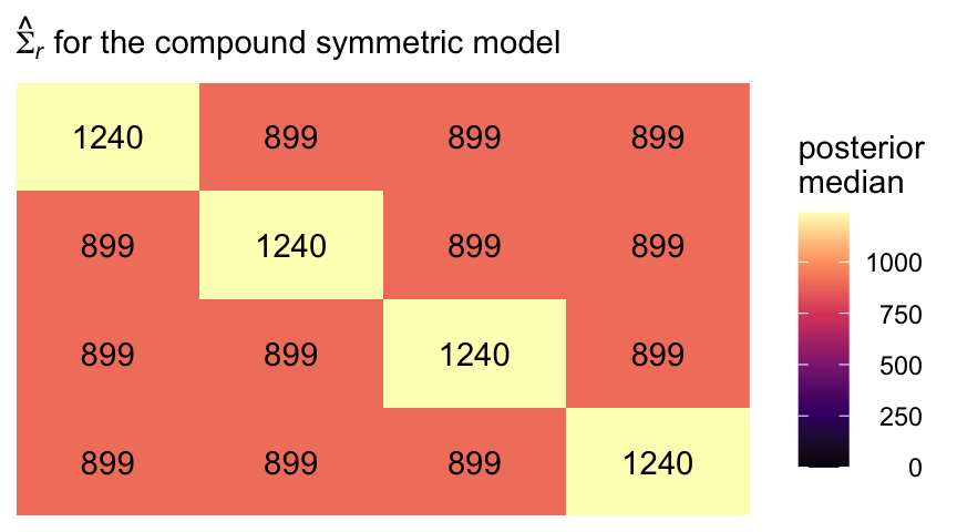
To simplify, we might pull the posterior medians for \(\sigma^2 + \sigma_1^2\) and \(\sigma_1^2\). We’ll call them diagonal and off_diagonal, respectively.

diagonal <- median(sigma.cs$`sigma^2 + sigma[1]^2`)
off_diagonal <- median(sigma.cs$`sigma[1]^2`)

Now we have them, we can make our colored version of the \(\mathbf{\Sigma}_r\) Singer and Willett reported in the rightmost column of Table 7.3.

crossing(row = 1:4,
         col = factor(1:4)) %>% 
  mutate(value = if_else(row == col, diagonal, off_diagonal)) %>% 
  mutate(label = round(value, digits = 0),
         col = fct_rev(col)) %>% 
  
  ggplot(aes(x = row, y = col)) +
  geom_tile(aes(fill = value)) +
  geom_text(aes(label = label)) +
  scale_fill_viridis_c("posterior\nmedian", option = "A", limits = c(0, NA)) +
  scale_x_continuous(NULL, breaks = NULL, position = "top", expand = c(0, 0)) +
  scale_y_discrete(NULL, breaks = NULL, expand = c(0, 0)) +
  labs(subtitle = expression(hat(Sigma)[italic(r)]*" for the compound symmetric model")) +
  theme(legend.text = element_text(hjust = 1))

7.3.3 Heterogeneous compound symmetric error covariance matrix

Now we extend the compound symmetric matrix by allowing the residual variances to vary across the time waves. Thus, instead of a single \(\sigma_\epsilon^2\) parameter, we’ll have \(\sigma_1^2\) through \(\sigma_4^2\). However, we still have a single correlation parameter \(\rho\). We can express this as

\[ \begin{align} \mathbf{\Sigma}_r & = \begin{bmatrix} \sigma_1^2 & \sigma_1 \sigma_2 \rho & \sigma_1 \sigma_3 \rho & \sigma_1 \sigma_4 \rho \\ \sigma_2 \sigma_1 \rho & \sigma_1^2 & \sigma_2 \sigma_3 \rho & \sigma_2 \sigma_4 \rho \\ \sigma_3 \sigma_1 \rho & \sigma_3 \sigma_2 \rho & \sigma_3^2 & \sigma_3 \sigma_4 \rho \\ \sigma_4 \sigma_1 \rho & \sigma_4 \sigma_2 \rho & \sigma_4 \sigma_3 \rho & \sigma_4^2 \end{bmatrix}, \end{align} \]

where, even though the correlation is the same in all cells, the covariances will differ because they are based on different combinations of the \(\sigma\) parameters. To fit this model with brms, we will continue to use cosy(gr = id). But now we wrap the entire model formula within the bf() function and allow the residual standard deviations to vary across he waves with the line sigma ~ 0 + factor(time).

fit7.4 <- brm(
  data = opposites_pp,
  family = gaussian,
  bf(opp ~ 0 + Intercept + time + ccog + time:ccog + cosy(gr = id),
     sigma ~ 0 + factor(time)), 
  iter = 2000, warmup = 1000, chains = 4, cores = 4,
  seed = 7,
  file = "fits/fit07.04")

Check the summary.

print(fit7.4, digits = 3)
 Family: gaussian 
  Links: mu = identity; sigma = log 
Formula: opp ~ 0 + Intercept + time + ccog + time:ccog + cosy(gr = id) 
         sigma ~ 0 + factor(time)
   Data: opposites_pp (Number of observations: 140) 
  Draws: 4 chains, each with iter = 2000; warmup = 1000; thin = 1;
         total post-warmup draws = 4000

Correlation Structures:
     Estimate Est.Error l-95% CI u-95% CI  Rhat Bulk_ESS Tail_ESS
cosy    0.720     0.060    0.592    0.830 1.005     1704     1837

Regression Coefficients:
                  Estimate Est.Error l-95% CI u-95% CI  Rhat Bulk_ESS Tail_ESS
Intercept          164.415     5.682  153.560  175.795 1.000     3690     2738
time                26.905     1.502   23.950   29.849 1.002     3800     2933
ccog                -0.179     0.463   -1.085    0.718 1.002     3251     2619
time:ccog            0.440     0.118    0.213    0.673 1.002     3958     2884
sigma_factortime0    3.641     0.124    3.417    3.902 1.005     2012     2178
sigma_factortime1    3.494     0.119    3.272    3.742 1.003     1843     2362
sigma_factortime2    3.529     0.121    3.306    3.774 1.002     2065     2370
sigma_factortime3    3.593     0.125    3.361    3.853 1.003     1955     2295

Draws were sampled using sampling(NUTS). For each parameter, Bulk_ESS
and Tail_ESS are effective sample size measures, and Rhat is the potential
scale reduction factor on split chains (at convergence, Rhat = 1).

If you look at the second row in the output, you’ll see that the brms default was to model \(\log(\sigma_j)\). Thus, you’ll have to exponentiate those posteriors to get them in their natural metric. Here’s a quick conversion.

fixef(fit7.4)[5:8, -2] %>% exp()
                  Estimate     Q2.5    Q97.5
sigma_factortime0 38.14764 30.48905 49.51246
sigma_factortime1 32.91011 26.35654 42.19741
sigma_factortime2 34.10152 27.28920 43.53938
sigma_factortime3 36.34854 28.81602 47.13603

To get the marginal posteriors for the full \(\mathbf{\Sigma}_r\) matrix, we’ll want to work directly with the output from as_draws_df().

sigma.hcs <- as_draws_df(fit7.4) %>%
  transmute(`sigma[1]`   = exp(b_sigma_factortime0),
            `sigma[2]`   = exp(b_sigma_factortime1),
            `sigma[3]`   = exp(b_sigma_factortime2),
            `sigma[4]`   = exp(b_sigma_factortime3),
            
            rho          = cosy,
            
            `sigma[1]^2` = exp(b_sigma_factortime0)^2,
            `sigma[2]^2` = exp(b_sigma_factortime1)^2,
            `sigma[3]^2` = exp(b_sigma_factortime2)^2,
            `sigma[4]^2` = exp(b_sigma_factortime3)^2) %>% 
  mutate(`sigma[2]*sigma[1]*rho` = `sigma[2]` * `sigma[1]` * rho,
         `sigma[3]*sigma[1]*rho` = `sigma[3]` * `sigma[1]` * rho,
         `sigma[4]*sigma[1]*rho` = `sigma[4]` * `sigma[1]` * rho,
         
         `sigma[1]*sigma[2]*rho` = `sigma[1]` * `sigma[2]` * rho,
         `sigma[3]*sigma[2]*rho` = `sigma[3]` * `sigma[2]` * rho,
         `sigma[4]*sigma[2]*rho` = `sigma[4]` * `sigma[2]` * rho,
         
         `sigma[1]*sigma[3]*rho` = `sigma[1]` * `sigma[3]` * rho,
         `sigma[2]*sigma[3]*rho` = `sigma[2]` * `sigma[3]` * rho,
         `sigma[4]*sigma[3]*rho` = `sigma[4]` * `sigma[3]` * rho,
         
         `sigma[1]*sigma[4]*rho` = `sigma[1]` * `sigma[4]` * rho,
         `sigma[2]*sigma[4]*rho` = `sigma[2]` * `sigma[4]` * rho,
         `sigma[3]*sigma[4]*rho` = `sigma[3]` * `sigma[4]` * rho)

# what did we do?
glimpse(sigma.hcs)
Rows: 4,000
Columns: 21
$ `sigma[1]`              <dbl> 35.56208, 35.57836, 33.08933, 40.70314, 30.48914, 32.99203, 37.94815, 34.25566, 35.42878, 35.996…
$ `sigma[2]`              <dbl> 33.89407, 27.96338, 30.16567, 31.72296, 29.12656, 31.00532, 30.26289, 32.73009, 26.74998, 29.142…
$ `sigma[3]`              <dbl> 32.12802, 32.03955, 28.60996, 33.40432, 29.84702, 30.76859, 35.32730, 28.68270, 28.11751, 26.272…
$ `sigma[4]`              <dbl> 35.59806, 32.35704, 35.97292, 35.62483, 35.83509, 35.78706, 38.32063, 30.29754, 29.57775, 29.713…
$ rho                     <dbl> 0.6875016, 0.6944474, 0.6521933, 0.6996793, 0.6928762, 0.7100510, 0.7489264, 0.5943043, 0.684699…
$ `sigma[1]^2`            <dbl> 1264.6614, 1265.8195, 1094.9037, 1656.7458, 929.5879, 1088.4742, 1440.0624, 1173.4503, 1255.1984…
$ `sigma[2]^2`            <dbl> 1148.8083, 781.9504, 909.9677, 1006.3460, 848.3564, 961.3296, 915.8427, 1071.2586, 715.5612, 849…
$ `sigma[3]^2`            <dbl> 1032.2095, 1026.5327, 818.5296, 1115.8487, 890.8449, 946.7061, 1248.0183, 822.6971, 790.5946, 69…
$ `sigma[4]^2`            <dbl> 1267.2221, 1046.9782, 1294.0513, 1269.1287, 1284.1537, 1280.7136, 1468.4711, 917.9409, 874.8432,…
$ `sigma[2]*sigma[1]*rho` <dbl> 828.6758, 690.8995, 650.9944, 903.4427, 615.3044, 726.3313, 860.0828, 666.3285, 648.9028, 699.77…
$ `sigma[3]*sigma[1]*rho` <dbl> 785.4975, 791.6107, 617.4211, 951.3265, 630.5244, 720.7857, 1004.0152, 583.9306, 682.0767, 630.8…
$ `sigma[4]*sigma[1]*rho` <dbl> 870.3366, 799.4551, 776.3187, 1014.5648, 757.0235, 838.3485, 1089.0868, 616.8060, 717.4991, 713.…
$ `sigma[1]*sigma[2]*rho` <dbl> 828.6758, 690.8995, 650.9944, 903.4427, 615.3044, 726.3313, 860.0828, 666.3285, 648.9028, 699.77…
$ `sigma[3]*sigma[2]*rho` <dbl> 748.6545, 622.1790, 562.8679, 741.4388, 602.3458, 677.3814, 800.6820, 557.9252, 514.9919, 510.74…
$ `sigma[4]*sigma[2]*rho` <dbl> 829.5143, 628.3445, 707.7259, 790.7251, 723.1915, 787.8648, 868.5249, 589.3366, 541.7371, 577.63…
$ `sigma[1]*sigma[3]*rho` <dbl> 785.4975, 791.6107, 617.4211, 951.3265, 630.5244, 720.7857, 1004.0152, 583.9306, 682.0767, 630.8…
$ `sigma[2]*sigma[3]*rho` <dbl> 748.6545, 622.1790, 562.8679, 741.4388, 602.3458, 677.3814, 800.6820, 557.9252, 514.9919, 510.74…
$ `sigma[4]*sigma[3]*rho` <dbl> 786.2923, 719.9372, 671.2268, 832.6347, 741.0801, 781.8494, 1013.8701, 516.4594, 569.4323, 520.7…
$ `sigma[1]*sigma[4]*rho` <dbl> 870.3366, 799.4551, 776.3187, 1014.5648, 757.0235, 838.3485, 1089.0868, 616.8060, 717.4991, 713.…
$ `sigma[2]*sigma[4]*rho` <dbl> 829.5143, 628.3445, 707.7259, 790.7251, 723.1915, 787.8648, 868.5249, 589.3366, 541.7371, 577.63…
$ `sigma[3]*sigma[4]*rho` <dbl> 786.2923, 719.9372, 671.2268, 832.6347, 741.0801, 781.8494, 1013.8701, 516.4594, 569.4323, 520.7…

Here’s the numeric summary.

sigma.hcs %>% 
  pivot_longer(everything()) %>% 
  group_by(name) %>% 
  median_qi(value) %>% 
  mutate_if(is.double, round, digits = 2)
# A tibble: 21 × 7
   name                    value .lower  .upper .width .point .interval
   <chr>                   <dbl>  <dbl>   <dbl>  <dbl> <chr>  <chr>    
 1 rho                      0.72   0.59    0.83   0.95 median qi       
 2 sigma[1]                38.0   30.5    49.5    0.95 median qi       
 3 sigma[1]*sigma[2]*rho  896.   535.   1609.     0.95 median qi       
 4 sigma[1]*sigma[3]*rho  930.   556.   1655.     0.95 median qi       
 5 sigma[1]*sigma[4]*rho  990.   589.   1795.     0.95 median qi       
 6 sigma[1]^2            1447.   930.   2451.     0.95 median qi       
 7 sigma[2]                32.8   26.4    42.2    0.95 median qi       
 8 sigma[2]*sigma[1]*rho  896.   535.   1609.     0.95 median qi       
 9 sigma[2]*sigma[3]*rho  796.   479.   1425.     0.95 median qi       
10 sigma[2]*sigma[4]*rho  853.   509.   1517.     0.95 median qi       
# ℹ 11 more rows

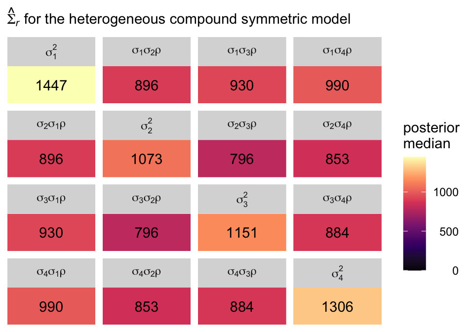
That’s a lot of information to wade through. Here we simplify the picture by making our plot version of the matrix Singer and Willett reported in the rightmost column of Table 7.3.

# arrange the panels
levels <- c(
  "sigma[1]^2", "sigma[1]*sigma[2]*rho", "sigma[1]*sigma[3]*rho", "sigma[1]*sigma[4]*rho", 
  "sigma[2]*sigma[1]*rho", "sigma[2]^2", "sigma[2]*sigma[3]*rho", "sigma[2]*sigma[4]*rho", 
  "sigma[3]*sigma[1]*rho", "sigma[3]*sigma[2]*rho", "sigma[3]^2", "sigma[3]*sigma[4]*rho", 
  "sigma[4]*sigma[1]*rho", "sigma[4]*sigma[2]*rho", "sigma[4]*sigma[3]*rho", "sigma[4]^2")


sigma.hcs %>% 
  select(`sigma[1]^2`:`sigma[3]*sigma[4]*rho`) %>% 
  pivot_longer(everything()) %>%  
  mutate(name = factor(name, levels = levels)) %>% 
  group_by(name) %>% 
  median_qi(value) %>% 
  mutate(label = round(value, digits = 0)) %>% 
  
  ggplot(aes(x = 0, y = 0)) +
  geom_tile(aes(fill = value)) +
  geom_text(aes(label = label)) +
  scale_fill_viridis_c("posterior\nmedian", option = "A", limits = c(0, NA)) +
  scale_x_continuous(NULL, breaks = NULL, expand = c(0, 0)) +
  scale_y_continuous(NULL, breaks = NULL, expand = c(0, 0)) +
  labs(subtitle = expression(hat(Sigma)[italic(r)]*" for the heterogeneous compound symmetric model")) +
  theme(legend.text = element_text(hjust = 1)) +
  facet_wrap(~ name, labeller = label_parsed)

7.3.4 Autoregressive error covariance matrix

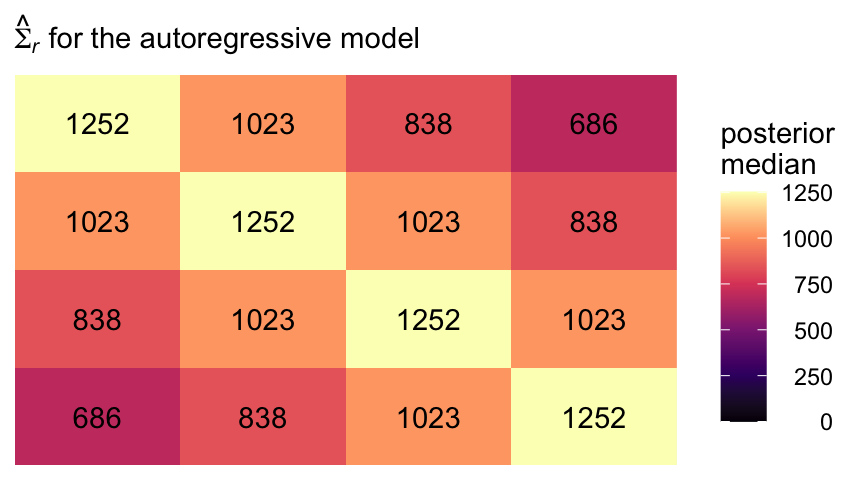
The first-order autoregressive has a strict “band-diagonal” structure governed by two parameters, which Singer and Willett called \(\sigma^2\) and \(\rho\). From Table 7.3 (p. 260), we see that matrix follows the form

\[ \begin{align} \mathbf{\Sigma}_r & = \begin{bmatrix} \sigma^2 & \sigma^2 \rho & \sigma^2 \rho^2 & \sigma^2 \rho^3 \\ \sigma^2 \rho & \sigma^2 & \sigma^2 \rho & \sigma^2 \rho^2 \\ \sigma^2 \rho^2 & \sigma^2 \rho & \sigma^2 & \sigma^2 \rho \\ \sigma^2 \rho^3 & \sigma^2 \rho^2 & \sigma^2 \rho & \sigma^2 \end{bmatrix}, \end{align} \]

where \(\rho\) is the correlation of one time point to the one immediately before or after, after conditioning on the liner model. In a similar way, \(\rho^2\) is the correlation between time points with one degree of separation (e.g., time 1 with time 3) and \(\rho^3\) is the correlation between the first and fourth time point. The other parameter, \(\sigma^2\) is the residual variance after conditioning on the linear model.

Once can fit this model with brms using a version of the ar() syntax. However, the model will follow a slightly different parameterization, following the form:

\[ \begin{align} \mathbf{\Sigma}_r & = \begin{bmatrix} \left (\sigma_\epsilon \Big / \sqrt{1 - \rho^2} \right )^2 & \left (\sigma_\epsilon \Big / \sqrt{1 - \rho^2} \right )^2 \rho & \left (\sigma_\epsilon \Big / \sqrt{1 - \rho^2} \right )^2 \rho^2 & \left (\sigma_\epsilon \Big / \sqrt{1 - \rho^2} \right )^2 \rho^3 \\ \left (\sigma_\epsilon \Big / \sqrt{1 - \rho^2} \right )^2 \rho & \left (\sigma_\epsilon \Big / \sqrt{1 - \rho^2} \right )^2 & \left (\sigma_\epsilon \Big / \sqrt{1 - \rho^2} \right )^2 \rho & \left (\sigma_\epsilon \Big / \sqrt{1 - \rho^2} \right )^2 \rho^2 \\ \left (\sigma_\epsilon \Big / \sqrt{1 - \rho^2} \right )^2 \rho^2 & \left (\sigma_\epsilon \Big / \sqrt{1 - \rho^2} \right )^2 \rho & \left (\sigma_\epsilon \Big / \sqrt{1 - \rho^2} \right )^2 & \left (\sigma_\epsilon \Big / \sqrt{1 - \rho^2} \right )^2 \rho \\ \left (\sigma_\epsilon \Big / \sqrt{1 - \rho^2} \right )^2 \rho^3 & \left (\sigma_\epsilon \Big / \sqrt{1 - \rho^2} \right )^2 \rho^2 & \left (\sigma_\epsilon \Big / \sqrt{1 - \rho^2} \right )^2 \rho & \left (\sigma_\epsilon \Big / \sqrt{1 - \rho^2} \right )^2 \end{bmatrix},\\ \end{align} \]

where \(\sigma_\epsilon\) is the residual variance after conditioning on both the linear model AND the autoregressive correlation \(\rho\). It’s not clear to me why brms is parameterized this way, but this is what we’ve got. The main point to get is that what Singer and Willett called \(\sigma\) in their autoregressive model, we’ll have to call \(\sigma_\epsilon \Big / \sqrt{1 - \rho^2}\). Thus, if you substitute our verbose brms term \(\sigma_\epsilon \Big / \sqrt{1 - \rho^2}\) for Singer and Willett’s compact term \(\sigma\), you’ll see the hellish matrix above is the same as the much simpler one before it.

To fit the first-order autoregressive model with brms, we use the ar() function. As with the last few models, notice how we continue to omit the (1 + time | id) syntax. Instead, we impose the autoregressive structure within persons by setting gr = id within ar(). We also set cov = TRUE.

fit7.5 <- brm(
  data = opposites_pp,
  family = gaussian,
  opp ~ 0 + Intercept + time + ccog + time:ccog + ar(gr = id, cov = TRUE),
  iter = 2000, warmup = 1000, chains = 4, cores = 4,
  seed = 7,
  file = "fits/fit07.05")

Check the summary.

print(fit7.5, digits = 3)
 Family: gaussian 
  Links: mu = identity 
Formula: opp ~ 0 + Intercept + time + ccog + time:ccog + ar(gr = id, cov = TRUE) 
   Data: opposites_pp (Number of observations: 140) 
  Draws: 4 chains, each with iter = 2000; warmup = 1000; thin = 1;
         total post-warmup draws = 4000

Correlation Structures:
      Estimate Est.Error l-95% CI u-95% CI  Rhat Bulk_ESS Tail_ESS
ar[1]    0.816     0.041    0.731    0.888 1.001     4530     3265

Regression Coefficients:
          Estimate Est.Error l-95% CI u-95% CI  Rhat Bulk_ESS Tail_ESS
Intercept  164.193     6.037  152.037  176.006 1.000     4923     3328
time        27.227     1.856   23.603   30.875 1.000     5013     3664
ccog        -0.039     0.480   -0.998    0.899 1.000     5030     3189
time:ccog    0.423     0.152    0.118    0.727 1.000     5223     3356

Further Distributional Parameters:
      Estimate Est.Error l-95% CI u-95% CI  Rhat Bulk_ESS Tail_ESS
sigma   20.316     1.395   17.797   23.198 1.002     4379     3131

Draws were sampled using sampling(NUTS). For each parameter, Bulk_ESS
and Tail_ESS are effective sample size measures, and Rhat is the potential
scale reduction factor on split chains (at convergence, Rhat = 1).

The ar[1] row in our summary is \(\rho\). As we discussed just before fitting the model, the sigma line is the summary for what I’m calling \(\sigma_\epsilon\), which is the residual standard deviation after conditioning on both the linear model AND \(\rho\). If we rename the \(\sigma^2\) parameter in the text as \(\sigma_\text{Singer \& Willett (2003)}^2\), we can convert our \(\sigma_\epsilon\) parameter to that metric using the formula

\[\sigma_\text{Singer \& Willett (2003)}^2 = \left (\sigma_\epsilon \Big / \sqrt{1 - \rho^2} \right )^2.\]

With that formula in hand, we’re ready to compute the marginal posteriors for the full \(\mathbf{\Sigma}_r\) matrix, saving the results as sigma.ar.

sigma.ar <- as_draws_df(fit7.5) %>% 
  mutate(sigma_e = sigma,
         sigma   = sigma_e / sqrt(1 - `ar[1]`^2)) %>% 
  transmute(rho             = `ar[1]`,
            `sigma^2`       = sigma^2,
            `sigma^2 rho`   = sigma^2 * rho,
            `sigma^2 rho^2` = sigma^2 * rho^2,
            `sigma^2 rho^3` = sigma^2 * rho^3)

Here’s the numeric summary.

sigma.ar %>% 
  pivot_longer(everything()) %>% 
  group_by(name) %>% 
  median_qi(value) %>% 
  mutate_if(is.double, round, digits = 2)
# A tibble: 5 × 7
  name            value .lower  .upper .width .point .interval
  <chr>           <dbl>  <dbl>   <dbl>  <dbl> <chr>  <chr>    
1 rho              0.82   0.73    0.89   0.95 median qi       
2 sigma^2       1252.   890.   1912.     0.95 median qi       
3 sigma^2 rho   1023.   668.   1664.     0.95 median qi       
4 sigma^2 rho^2  838.   496.   1471.     0.95 median qi       
5 sigma^2 rho^3  686.   365.   1298.     0.95 median qi       

To simplify, we might pull the posterior medians for \(\sigma^2\) through \(\sigma^2 \rho^3\).

s2   <- median(sigma.ar$`sigma^2`)
s2p  <- median(sigma.ar$`sigma^2 rho`)
s2p2 <- median(sigma.ar$`sigma^2 rho^2`)
s2p3 <- median(sigma.ar$`sigma^2 rho^3`)

Now we have them, we can make our colored version of the \(\mathbf{\Sigma}_r\) Singer and Willett reported in the rightmost column of Table 7.3.

crossing(row = 1:4,
         col = factor(1:4)) %>% 
  mutate(value = c(s2, s2p, s2p2, s2p3,
                   s2p, s2, s2p, s2p2,
                   s2p2, s2p, s2, s2p,
                   s2p3, s2p2, s2p, s2)) %>% 
  mutate(label = round(value, digits = 0),
         col   = fct_rev(col)) %>% 
  
  ggplot(aes(x = row, y = col)) +
  geom_tile(aes(fill = value)) +
  geom_text(aes(label = label)) +
  scale_fill_viridis_c("posterior\nmedian", option = "A", limits = c(0, NA)) +
  scale_x_continuous(NULL, breaks = NULL, position = "top", expand = c(0, 0)) +
  scale_y_discrete(NULL, breaks = NULL, expand = c(0, 0)) +
  labs(subtitle = expression(hat(Sigma)[italic(r)]*" for the autoregressive model")) +
  theme(legend.text = element_text(hjust = 1))

With this presentation, that strict band-diagonal structure really pops.

7.3.5 Heterogeneous autoregressive error covariance matrix

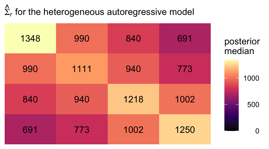
For the heterogeneous autoregressive error covariance matrix, we relax the assumption that the variances on the diagonal of the \(\mathbf{\Sigma}_r\) matrix are constant across waves. From Table 7.3 (p. 260), we see that matrix follows the form

\[ \begin{align} \mathbf{\Sigma}_r & = \begin{bmatrix} \sigma_1^2 & \sigma_1 \sigma_2 \rho & \sigma_1 \sigma_3 \rho^2 & \sigma_1 \sigma_4 \rho^3 \\ \sigma_2 \sigma_1 \rho & \sigma_2^2 & \sigma_2 \sigma_3 \rho & \sigma_2 \sigma_4 \rho^2 \\ \sigma_3 \sigma_1 \rho^2 & \sigma_3 \sigma_2 \rho & \sigma_3^2 & \sigma_3 \sigma_4 \rho \\ \sigma_4 \sigma_1 \rho^3 & \sigma_4 \sigma_2 \rho^2 & \sigma_4 \sigma_3 \rho & \sigma_4^2 \end{bmatrix}, \end{align} \]

where, as before, \(\rho\) is the correlation of one time point to the one immediately before or after, after conditioning on the liner model. To fit this model with brms, we continue to use the ar(gr = id, cov = TRUE) syntax. The only adjustment is we now wrap the formula within the bf() function and add a second line for sigma.

fit7.6 <- brm(
  data = opposites_pp,
  family = gaussian,
  bf(opp ~ 0 + Intercept + time + ccog + time:ccog + ar(gr = id, cov = TRUE),
     sigma ~ 0 + factor(time)), 
  iter = 2000, warmup = 1000, chains = 4, cores = 4,
  seed = 7,
  file = "fits/fit07.06")

Inspect the parameter summary.

print(fit7.6, digits = 3)
 Family: gaussian 
  Links: mu = identity; sigma = log 
Formula: opp ~ 0 + Intercept + time + ccog + time:ccog + ar(gr = id, cov = TRUE) 
         sigma ~ 0 + factor(time)
   Data: opposites_pp (Number of observations: 140) 
  Draws: 4 chains, each with iter = 2000; warmup = 1000; thin = 1;
         total post-warmup draws = 4000

Correlation Structures:
      Estimate Est.Error l-95% CI u-95% CI  Rhat Bulk_ESS Tail_ESS
ar[1]    0.808     0.043    0.715    0.884 1.000     4091     3167

Regression Coefficients:
                  Estimate Est.Error l-95% CI u-95% CI  Rhat Bulk_ESS Tail_ESS
Intercept          164.639     6.156  152.417  176.771 1.000     4077     3125
time                27.139     2.002   23.248   31.070 1.000     4145     3300
ccog                -0.119     0.504   -1.079    0.893 1.002     3979     2731
time:ccog            0.428     0.160    0.110    0.738 1.002     4262     3212
sigma_factortime0    3.066     0.102    2.874    3.279 1.001     3738     3018
sigma_factortime1    2.967     0.086    2.810    3.143 1.000     3266     2883
sigma_factortime2    3.012     0.085    2.856    3.191 1.001     3777     3029
sigma_factortime3    3.026     0.102    2.838    3.238 1.000     3885     3633

Draws were sampled using sampling(NUTS). For each parameter, Bulk_ESS
and Tail_ESS are effective sample size measures, and Rhat is the potential
scale reduction factor on split chains (at convergence, Rhat = 1).

Here are summaries for the four \(\sigma_\epsilon\) posteriors, after exponentiation.

fixef(fit7.6)[5:8, -2] %>% exp()
                  Estimate     Q2.5    Q97.5
sigma_factortime0 21.44741 17.70577 26.54369
sigma_factortime1 19.44305 16.60763 23.17069
sigma_factortime2 20.33684 17.39643 24.31242
sigma_factortime3 20.62398 17.07822 25.47298

Extending our workflow from the last section, here how we might compute the marginal posteriors for the full \(\mathbf{\Sigma}_r\) matrix, saving the results as sigma.har.

sigma.har <- as_draws_df(fit7.6) %>% 
  mutate(sigma_1e = exp(b_sigma_factortime0),
         sigma_2e = exp(b_sigma_factortime1),
         sigma_3e = exp(b_sigma_factortime2),
         sigma_4e = exp(b_sigma_factortime3)) %>% 
  mutate(sigma_1 = sigma_1e / sqrt(1 - `ar[1]`^2),
         sigma_2 = sigma_2e / sqrt(1 - `ar[1]`^2),
         sigma_3 = sigma_3e / sqrt(1 - `ar[1]`^2),
         sigma_4 = sigma_4e / sqrt(1 - `ar[1]`^2)) %>% 
  transmute(rho = `ar[1]`,
            
            `sigma_1^2` = sigma_1^2,
            `sigma_2^2` = sigma_2^2,
            `sigma_3^2` = sigma_3^2,
            `sigma_4^2` = sigma_4^2,
            
            `sigma_2 sigma_1 rho`   = sigma_2 * sigma_1 * rho,
            `sigma_3 sigma_1 rho^2` = sigma_3 * sigma_1 * rho^2,
            `sigma_4 sigma_1 rho^3` = sigma_4 * sigma_1 * rho^3,
            `sigma_3 sigma_2 rho`   = sigma_3 * sigma_2 * rho,
            `sigma_4 sigma_2 rho^2` = sigma_4 * sigma_2 * rho^2,
            `sigma_4 sigma_3 rho`   = sigma_4 * sigma_3 * rho)

Here’s the numeric summary.

sigma.har %>% 
  pivot_longer(everything()) %>% 
  group_by(name) %>% 
  median_qi(value) %>% 
  mutate_if(is.double, round, digits = 2)
# A tibble: 11 × 7
   name                    value .lower  .upper .width .point .interval
   <chr>                   <dbl>  <dbl>   <dbl>  <dbl> <chr>  <chr>    
 1 rho                      0.81   0.72    0.88   0.95 median qi       
 2 sigma_1^2             1348.   876.   2204.     0.95 median qi       
 3 sigma_2 sigma_1 rho    990.   626.   1684.     0.95 median qi       
 4 sigma_2^2             1111.   724.   1821.     0.95 median qi       
 5 sigma_3 sigma_1 rho^2  840.   480.   1516.     0.95 median qi       
 6 sigma_3 sigma_2 rho    940.   569.   1614.     0.95 median qi       
 7 sigma_3^2             1218.   775.   2042.     0.95 median qi       
 8 sigma_4 sigma_1 rho^3  691.   362.   1317.     0.95 median qi       
 9 sigma_4 sigma_2 rho^2  773.   439.   1415.     0.95 median qi       
10 sigma_4 sigma_3 rho   1002.   614.   1730.     0.95 median qi       
11 sigma_4^2             1250.   804.   2091      0.95 median qi       

As in the last section, we might pull the posterior medians for \(\sigma1^2\) through \(\sigma_4^2\).

s12   <- median(sigma.har$`sigma_1^2`)
s22   <- median(sigma.har$`sigma_2^2`)
s32   <- median(sigma.har$`sigma_3^2`)
s42   <- median(sigma.har$`sigma_4^2`)

s2s1p  <- median(sigma.har$`sigma_2 sigma_1 rho`)

s3s1p2 <- median(sigma.har$`sigma_3 sigma_1 rho^2`)
s3s2p  <- median(sigma.har$`sigma_3 sigma_2 rho`)

s4s1p3 <- median(sigma.har$`sigma_4 sigma_1 rho^3`)
s4s2p2 <- median(sigma.har$`sigma_4 sigma_2 rho^2`)
s4s3p  <- median(sigma.har$`sigma_4 sigma_3 rho`)

Now we have them, we can make our colored version of the \(\mathbf{\Sigma}_r\) Singer and Willett reported in the rightmost column of Table 7.3.

crossing(row = 1:4,
         col = factor(1:4)) %>% 
  mutate(value = c(s12, s2s1p, s3s1p2, s4s1p3,
                   s2s1p, s22, s3s2p, s4s2p2,
                   s3s1p2, s3s2p, s32, s4s3p,
                   s4s1p3, s4s2p2, s4s3p, s42)) %>% 
  mutate(label = round(value, digits = 0),
         col   = fct_rev(col)) %>% 
  
  ggplot(aes(x = row, y = col)) +
  geom_tile(aes(fill = value)) +
  geom_text(aes(label = label)) +
  scale_fill_viridis_c("posterior\nmedian", option = "A", limits = c(0, NA)) +
  scale_x_continuous(NULL, breaks = NULL, position = "top", expand = c(0, 0)) +
  scale_y_discrete(NULL, breaks = NULL, expand = c(0, 0)) +
  labs(subtitle = expression(hat(Sigma)[italic(r)]*" for the heterogeneous autoregressive model")) +
  theme(legend.text = element_text(hjust = 1))

Even though there’s still a strict band diagonal correlation structure, the heterogeneous variances allow for differences among the covariances within the bands.

7.3.6 Toeplitz error covariance matrix

Handy as it is, brms is not yet set up to fit models with the Toeplitz error covariance matrix, at this time. For details, see brms GitHub issue #403.

7.3.7 Does choosing the “correct” error covariance structure really matter?

Now we have all our models, we might compare them with information criteria, as was done in the text. Here we’ll use the WAIC. First, compute and save the WAIC estimates.

fit7.1 <- add_criterion(fit7.1, criterion = "waic")
fit7.2 <- add_criterion(fit7.2, criterion = "waic")
fit7.3 <- add_criterion(fit7.3, criterion = "waic")
fit7.4 <- add_criterion(fit7.4, criterion = "waic")
fit7.5 <- add_criterion(fit7.5, criterion = "waic")
fit7.6 <- add_criterion(fit7.6, criterion = "waic")

Now compare the models using WAIC differences and WAIC weights.

loo_compare(fit7.1, fit7.2, fit7.3, fit7.4, fit7.5, fit7.6, criterion = "waic") %>% print(simplify = F)
       elpd_diff se_diff elpd_waic se_elpd_waic p_waic se_p_waic waic   se_waic
fit7.1    0.0       0.0  -586.7       6.2         47.1    3.5    1173.5   12.3 
fit7.5  -20.9       4.1  -607.7       8.5          3.4    0.5    1215.4   17.1 
fit7.2  -21.5       2.8  -608.2       7.6         14.2    1.7    1216.4   15.3 
fit7.6  -23.7       4.2  -610.5       8.8          6.7    1.1    1220.9   17.6 
fit7.3  -39.5       5.9  -626.2       8.1          4.5    0.7    1252.5   16.3 
fit7.4  -41.4       5.4  -628.1       7.8          7.0    0.8    1256.2   15.6 
model_weights(fit7.1, fit7.2, fit7.3, fit7.4, fit7.5, fit7.6, weights = "waic") %>% round(digits = 3)
fit7.1 fit7.2 fit7.3 fit7.4 fit7.5 fit7.6 
     1      0      0      0      0      0 

By both methods of comparison, the standard multilevel model for change was the clear winner.

Perhaps most important, consider how choice of an error covariance structure affects our ability to address our research questions, especially given that it is the fixed effects–and not the variance components–that usually embody these questions. Some might say that refining the error covariance structure for the multilevel model for change is akin to rearranging the deck chairs on the Titanic–it rarely fundamentally changes our parameter estimates. Indeed, regardless of the error structure chosen, estimates of the fixed effects are unbiased and may not be affected much by choices made in the stochastic part of the model (providing that neither the data, nor the error structure, are idiosyncratic). (p. 264, emphasis in the original)

For more on the idea that researchers generally just care about fixed effects, see the paper by McNeish et al. (2017), On the unnecessary ubiquity of hierarchical linear modeling. Although I can’t disagree with the logic presented by Singer and Willett, or by McNeish and colleagues, I’m uneasy with this perspective for a couple reasons. First, I suspect part of the reason researchers don’t theorize about variances and covariances is because those are difficult metrics for many of us to think about. Happily, brms makes these more accessible by parameterizing them as standard deviations and correlations.

Second, in many disciplines, including my own (clinical psychology), multilevel models are still exotic and researchers just aren’t used to thinking in their terms. But I see this as more of a reason to spread the multilevel gospel than to down emphasize variance parameters. In my opinion, which is heavily influenced by McElreath’s, it would be great if someday soon, researchers used multilevel models (longitudinal or otherwise) as the default rather than the exception.

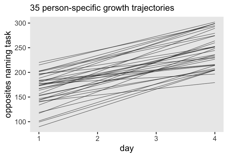
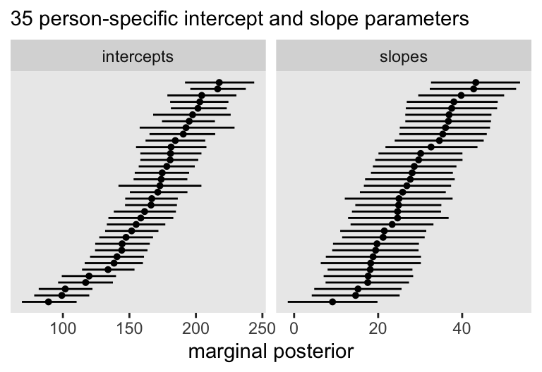
Third, I actually care about random effects. If you go back and compare the models from this chapter, it was only the multilevel growth model (fit7.1) that assigned person-specific intercepts and slopes. In clinical psychology, this matters! I want a model that allows me to make plots like this:

# 35 person-specific growth trajectories
nd <- opposites_pp %>% 
  distinct(id, ccog) %>% 
  expand(nesting(id, ccog),
         time = c(0, 3))

fitted(fit7.1, newdata = nd) %>% 
  data.frame() %>% 
  bind_cols(nd) %>% 
  ggplot(aes(x = time + 1, y = Estimate, group = id)) +
  geom_line(linewidth = 1/4, alpha = 2/3) +
  labs(subtitle = "35 person-specific growth trajectories",
       x = "day",
       y = "opposites naming task") +
  theme(panel.grid = element_blank())

# 35 person-specific intercept and slope parameters
rbind(coef(fit7.1)$id[, , "Intercept"],
      coef(fit7.1)$id[, , "time"]) %>% 
  data.frame() %>% 
  mutate(type = rep(c("intercepts", "slopes"), each = n() / 2)) %>% 
  group_by(type) %>% 
  arrange(Estimate) %>% 
  mutate(id = 1:35) %>% 
  
  ggplot(aes(x = Estimate, xmin = Q2.5, xmax = Q97.5, y = id)) +
  geom_pointrange(linewidth = 1/2, size = 1/10) +
  scale_y_continuous(NULL, breaks = NULL) +
  labs(subtitle = "35 person-specific intercept and slope parameters",
       x = "marginal posterior") +
  theme(panel.grid = element_blank()) +
  facet_wrap(~ type, scales = "free_x")

Of all the models we fit, only the standard multilevel model for change allows us to drill down all the way to the individual participants and this was accomplished by how it parameterized \(\mathbf{\Sigma}_r\). Even your substantive theory isn’t built around the subtleties in the \(4 \times 4 = 16\) cells in the \(\mathbf{\Sigma}_r\), it still matters that our fit7.1 parameterized them by way of \(\sigma_\epsilon\), \(\sigma_0\), \(\sigma_1\), and \(\rho_{01}\).

But Singer and Willett went on:

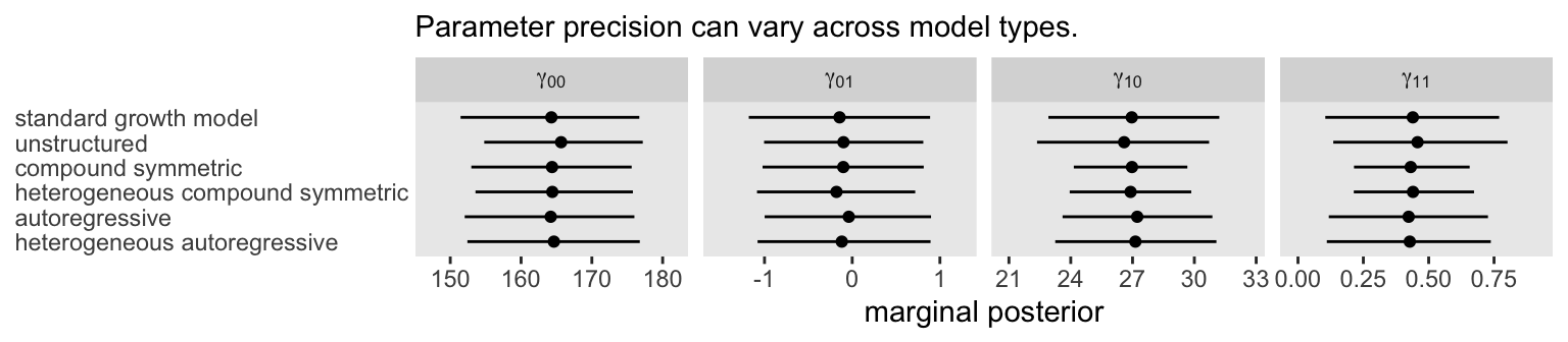
But refining our hypotheses about the error covariance structure does affect the precision of estimates of the fixed effects and will therefore impact hypothesis testing and confidence interval construction. (p. 264, emphasis in the original)

I’m going to showcase this in a coefficient plot, rather than the way the authors did in their Table 7.4. First, we’ll want a custom wrangling function. Let’s call it gamma_summary().

gamma_summary <- function(brmsfit) {
  fixef(brmsfit)[1:4, ] %>% 
    data.frame() %>% 
    mutate(gamma = c("gamma[0][0]", "gamma[1][0]", "gamma[0][1]", "gamma[1][1]"))
}

gamma_summary(fit7.1)
             Estimate Est.Error        Q2.5       Q97.5       gamma
Intercept 164.2819042 6.4642477 151.4539370 176.7035537 gamma[0][0]
time       26.9621087 2.0933771  22.9170354  31.2093872 gamma[1][0]
ccog       -0.1438951 0.5199258  -1.1788654   0.8879831 gamma[0][1]
time:ccog   0.4392846 0.1697978   0.1044915   0.7695013 gamma[1][1]

Now wrangle and plot.

type <- c(
  "standard growth model", "unstructured", "compound symmetric", 
  "heterogeneous compound symmetric", "autoregressive", "heterogeneous autoregressive")

tibble(fit  = str_c("fit7.", c(1:6)),
       type = factor(type, levels = type)) %>% 
  mutate(type  = fct_rev(type),
         gamma = map(fit, ~get(.) %>% gamma_summary())) %>% 
  unnest(gamma) %>% 
  
  ggplot(aes(x = Estimate, xmin = Q2.5, xmax = Q97.5, y = type)) +
  geom_pointrange(size = 1/5) +
  scale_x_continuous("marginal posterior", expand = expansion(mult = 0.25)) +
  labs(subtitle = "Parameter precision can vary across model types.",
       y = NULL) +
  theme(axis.text.y = element_text(hjust = 0),
        axis.ticks.y = element_blank(),
        panel.grid = element_blank()) +
  facet_wrap(~ gamma, scales = "free_x", labeller = label_parsed, nrow = 1)

Yep, the way we parameterize \(\mathbf{\Sigma}_r\) might have subtle consequences for the widths of our marginal \(\gamma\) posteriors. This can matter a lot when you’re analyzing data from, say, a clinical trial where lives may depend on the results of your analysis. Rearrange the deck chairs on your Titanic with caution, friends. Someone might trip and hurt themselves.

7.3.8 Bonus: Did we trade multilevel for multivariate?

So far in this chapter, only the first model fit7.1 used the conventional brms multilevel syntax, such as (1 + time | id). The other five models used the unstr(), cosy(), or ar() helper functions, instead. Singer and Willett didn’t exactly come out and say it this way, but in a sense, fit7.1 is the only multilevel model we’ve fit so far in this chapter. Mallinckrod et al. (2008) made the point more clearly:

A simple formulation of the general linear mixed model… can be implemented in which the random effects are not explicitly modeled, but rather are included as part of the marginal covariance matrix… leading them to what could alternatively be described as a multivariate normal model. (p. 306)

Thus we might think of all our models after fit7.1 as special kinds of multivariate panel models. To help make this easier to see, let’s first fit a simplified version of the unstructured model, following the form

\[ \begin{align} \text{opp}_{ij} & \sim \operatorname{Normal}(\mu_j, \mathbf{\Sigma}_r) \\ \mu_j & = \pi_{0j} \\ \mathbf{\Sigma}_r & = \begin{bmatrix} \sigma_1^2 & \sigma_{12} & \sigma_{13} & \sigma_{14} \\ \sigma_{21} & \sigma_2^2 & \sigma_{23} & \sigma_{24} \\ \sigma_{31} & \sigma_{32} & \sigma_3^2 & \sigma_{34} \\ \sigma_{41} & \sigma_{42} & \sigma_{43} & \sigma_4^2 \end{bmatrix}, \end{align} \]

where \(\pi_{0j}\) is the intercept, which is estimated separately for each of the 4 \(j\) time points, and \(\mathbf{\Sigma}_r\) is the unstructured variance/covariance matrix. To fit those separate \(\pi_{0j}\) intercepts with brm(), we use the syntax of 0 + factor(time) in the \(\mu_j\) portion of the model. Otherwise, the syntax is much the same as with the first unstructured model fit7.2.

fit7.7 <- brm(
  data = opposites_pp, 
  family = gaussian,
  bf(opp ~ 0 + factor(time) + unstr(time = time, gr = id),
     sigma ~ 0 + factor(time)),
  iter = 2000, warmup = 1000, chains = 4, cores = 4,
  seed = 7,
  file = "fits/fit07.07")

Check the parameter summary.

print(fit7.7, digits = 3)
 Family: gaussian 
  Links: mu = identity; sigma = log 
Formula: opp ~ 0 + factor(time) + unstr(time = time, gr = id) 
         sigma ~ 0 + factor(time)
   Data: opposites_pp (Number of observations: 140) 
  Draws: 4 chains, each with iter = 2000; warmup = 1000; thin = 1;
         total post-warmup draws = 4000

Correlation Structures:
             Estimate Est.Error l-95% CI u-95% CI  Rhat Bulk_ESS Tail_ESS
cortime(0,1)    0.739     0.077    0.563    0.859 1.001     2354     2259
cortime(0,2)    0.624     0.098    0.409    0.782 1.001     2037     2187
cortime(1,2)    0.780     0.065    0.628    0.883 1.000     2782     2943
cortime(0,3)    0.288     0.144   -0.015    0.545 1.001     2298     2515
cortime(1,3)    0.585     0.107    0.346    0.761 1.002     3050     2823
cortime(2,3)    0.735     0.077    0.555    0.857 1.001     3018     2793

Regression Coefficients:
                  Estimate Est.Error l-95% CI u-95% CI  Rhat Bulk_ESS Tail_ESS
factortime0        164.606     6.252  152.389  177.005 1.002     2387     2579
factortime1        192.099     5.528  180.967  202.933 1.001     2121     2114
factortime2        216.843     5.886  205.079  228.142 1.001     2046     1889
factortime3        246.174     6.432  233.158  258.451 1.001     2523     2876
sigma_factortime0    3.568     0.116    3.351    3.806 1.001     2785     3109
sigma_factortime1    3.460     0.112    3.251    3.690 1.001     2478     2365
sigma_factortime2    3.528     0.109    3.321    3.751 1.001     2239     2744
sigma_factortime3    3.613     0.116    3.404    3.850 1.001     2875     2784

Draws were sampled using sampling(NUTS). For each parameter, Bulk_ESS
and Tail_ESS are effective sample size measures, and Rhat is the potential
scale reduction factor on split chains (at convergence, Rhat = 1).

Once again, those 4 sigma_ parameters were fit using the log link. Here they are after exponentiation.

fixef(fit7.7)[5:8, -2] %>% exp()
                  Estimate     Q2.5    Q97.5
sigma_factortime0 35.45656 28.52038 44.97009
sigma_factortime1 31.82985 25.81269 40.04808
sigma_factortime2 34.05243 27.69567 42.56658
sigma_factortime3 37.08273 30.09709 47.00746

All we’ve really done is fit an unconditional multivariate normal model for opp, across the four time points. To see, compare the posterior point estimates in the Population-Level Effects section (or their exponentiated values, above), to the sample means and SD’s for opp over time.

opposites_pp %>% 
  group_by(time) %>% 
  summarise(m = mean(opp),
            s = sd(opp))
# A tibble: 4 × 3
   time     m     s
  <dbl> <dbl> <dbl>
1     0  164.  36.2
2     1  192   33.5
3     2  217.  35.9
4     3  246.  37.6

In a similar way, the correlations in the Correlation Structures part of the print() output are really just regularized sample correlations. Compare them to the un-regularized Pearson’s correlation estimates.

opposites_pp %>% 
  select(id, time, opp) %>% 
  pivot_wider(names_from = time, values_from = opp) %>% 
  select(-id) %>% 
  cor() %>% 
  round(digits = 3)
      0     1     2     3
0 1.000 0.804 0.709 0.414
1 0.804 1.000 0.847 0.678
2 0.709 0.847 1.000 0.800
3 0.414 0.678 0.800 1.000

The reason for the regularization, by the way, is because of the default LKJ(1) prior. That prior is more strongly regularizing as you increase the dimensions of the correlation matrix. In the case of a \(4 \times 4\) matrix, the LKJ will definitely push the individual correlations toward zero, particularly in the case of a modestly-sized data set like opposites_pp.

But anyway, we can fit basically the same model by explicitly using the brms multivariate syntax, as outlined in Bürkner’s (2022) vignette, Estimating multivariate models with brms. Before we can fit a more conventional multivariate model to the data, we’ll need to convert opposites_pp to the wide format, which we’ll call opposites_wide.

opposites_wide <- opposites_pp %>% 
  mutate(time = str_c("t", time)) %>% 
  select(-wave) %>% 
  pivot_wider(names_from = time, values_from = opp)

# what?
head(opposites_wide)
# A tibble: 6 × 7
     id   cog   ccog    t0    t1    t2    t3
  <dbl> <dbl>  <dbl> <dbl> <dbl> <dbl> <dbl>
1     1   137  23.5    205   217   268   302
2     2   123   9.54   219   243   279   302
3     3   129  15.5    142   212   250   289
4     4   125  11.5    206   230   248   273
5     5    81 -32.5    190   220   229   220
6     6   110  -3.46   165   205   207   263

Now we’re ready to fit a multivariate model to our 4 variables t0 through t3. To do so, we place all 4 variables within the mvbind() function, and we nest the entire model formula within the bf() function. Also notice we are explicitly asking for residual correlations by setting set_rescor(TRUE).

fit7.8 <- brm(
  data = opposites_wide, 
  family = gaussian,
  bf(mvbind(t0, t1, t2, t3) ~ 1) +
    set_rescor(TRUE),
  iter = 2000, warmup = 1000, chains = 4, cores = 4,
  seed = 7,
  file = "fits/fit07.08")

Review the model summary.

print(fit7.8, digits = 3)
 Family: MV(gaussian, gaussian, gaussian, gaussian) 
  Links: mu = identity
         mu = identity
         mu = identity
         mu = identity 
Formula: t0 ~ 1 
         t1 ~ 1 
         t2 ~ 1 
         t3 ~ 1 
   Data: opposites_wide (Number of observations: 35) 
  Draws: 4 chains, each with iter = 2000; warmup = 1000; thin = 1;
         total post-warmup draws = 4000

Regression Coefficients:
             Estimate Est.Error l-95% CI u-95% CI  Rhat Bulk_ESS Tail_ESS
t0_Intercept  164.516     5.807  152.990  176.136 1.001     2339     2617
t1_Intercept  192.037     5.210  181.789  201.859 1.001     2047     2374
t2_Intercept  216.789     5.630  205.493  227.683 1.001     1967     2313
t3_Intercept  246.113     6.292  233.689  258.336 1.000     2565     2718

Further Distributional Parameters:
         Estimate Est.Error l-95% CI u-95% CI  Rhat Bulk_ESS Tail_ESS
sigma_t0   35.805     4.109   28.956   45.091 1.000     2540     2826
sigma_t1   32.240     3.591   26.055   39.884 1.001     2103     2130
sigma_t2   34.425     3.851   27.758   42.555 1.000     2240     2692
sigma_t3   37.532     4.569   29.879   47.750 1.001     2610     2746

Residual Correlations: 
              Estimate Est.Error l-95% CI u-95% CI  Rhat Bulk_ESS Tail_ESS
rescor(t0,t1)    0.738     0.078    0.556    0.861 1.000     2183     2371
rescor(t0,t2)    0.624     0.101    0.397    0.790 1.000     2007     2291
rescor(t1,t2)    0.784     0.065    0.633    0.886 1.000     2613     3327
rescor(t0,t3)    0.288     0.147   -0.015    0.549 1.000     2343     2962
rescor(t1,t3)    0.590     0.105    0.357    0.770 1.000     2879     3158
rescor(t2,t3)    0.737     0.076    0.564    0.860 1.000     2884     2930

Draws were sampled using sampling(NUTS). For each parameter, Bulk_ESS
and Tail_ESS are effective sample size measures, and Rhat is the potential
scale reduction factor on split chains (at convergence, Rhat = 1).

The results are very similar to those for fit7.7, above, with a few small differences. First, we now have a Residual Correlations section instead of a Correlation Structures. The output of the two is basically the same, though. The various sigma_ parameters are now in their own Family Specific Parameters, instead of in the bottom fo the Population-Level Effects section. You’ll also note the sigma_ parameters are all in their natural metric, rather than the log metric. This is because, by default, brms used the log link for the syntax we used for fit7.7, but used the identity link for the syntax we used for fit7.8.

Even if you take these small formatting-type differences into account, a careful eye will notice the parameter summaries are still a little different between these two models. The reason is the defualt priors were a little different. Take a look:

fit7.7$prior
                prior    class        coef group resp  dpar nlpar lb ub tag       source
               (flat)        b                                                   default
               (flat)        b factortime0                                  (vectorized)
               (flat)        b factortime1                                  (vectorized)
               (flat)        b factortime2                                  (vectorized)
               (flat)        b factortime3                                  (vectorized)
               (flat)        b                        sigma                      default
               (flat)        b factortime0            sigma                 (vectorized)
               (flat)        b factortime1            sigma                 (vectorized)
               (flat)        b factortime2            sigma                 (vectorized)
               (flat)        b factortime3            sigma                 (vectorized)
 lkj_corr_cholesky(1) Lcortime                                                   default
fit7.8$prior
                   prior     class coef group resp dpar nlpar lb ub tag  source
 student_t(3, 166, 35.6) Intercept              t0                      default
   student_t(3, 196, 43) Intercept              t1                      default
 student_t(3, 215, 32.6) Intercept              t2                      default
 student_t(3, 246, 47.4) Intercept              t3                      default
    lkj_corr_cholesky(1)   Lrescor                                      default
   student_t(3, 0, 35.6)     sigma              t0             0        default
     student_t(3, 0, 43)     sigma              t1             0        default
   student_t(3, 0, 32.6)     sigma              t2             0        default
   student_t(3, 0, 47.4)     sigma              t3             0        default

I’m not going to break down exactly why brms made different default prior choices for these models, but experienced brms users should find these results very predictable, particularly due to our use of the 0 + factor(time) syntax in the fit7.7 model. Know your software defaults, friends. So let’s try fitting these two models one more time, but with a couple adjustments. First, we will explicitly set the priors based on the defaults used by fit7.8. We will manually request the identity link for the sigma_ parameters in fit7.7. We will also increase the post-warmup draws for both models, to help account for MCMC sampling error.

Now fit the models.

# unstructured
fit7.7b <- brm(
  data = opposites_pp, 
  family = brmsfamily(family = "gaussian", link = "identity", link_sigma = "identity"),
  bf(opp ~ 0 + factor(time) + unstr(time = time, gr = id),
     sigma ~ 0 + factor(time)),
  prior = c(prior(student_t(3, 166, 35.6), class = b, coef = factortime0),
            prior(student_t(3, 196, 43.0), class = b, coef = factortime1),
            prior(student_t(3, 215, 32.6), class = b, coef = factortime2),
            prior(student_t(3, 246, 47.4), class = b, coef = factortime3),
            
            prior(student_t(3, 0, 35.6), class = b, coef = factortime0, dpar = sigma),
            prior(student_t(3, 0, 43.0), class = b, coef = factortime1, dpar = sigma),
            prior(student_t(3, 0, 32.6), class = b, coef = factortime2, dpar = sigma),
            prior(student_t(3, 0, 47.4), class = b, coef = factortime3, dpar = sigma),
            
            prior(lkj(1), class = cortime)),
  iter = 13500, warmup = 1000, chains = 4, cores = 4,
  seed = 7,
  file = "fits/fit07.07b")

# multivariate
fit7.8b <- brm(
  data = opposites_wide, 
  family = gaussian,
  bf(mvbind(t0, t1, t2, t3) ~ 1) +
    set_rescor(TRUE),
  prior = c(prior(student_t(3, 166, 35.6), class = Intercept, resp = t0),
            prior(student_t(3, 196, 43.0), class = Intercept, resp = t1),
            prior(student_t(3, 215, 32.6), class = Intercept, resp = t2),
            prior(student_t(3, 246, 47.4), class = Intercept, resp = t3),
            
            prior(student_t(3, 0, 35.6), class = sigma, resp = t0),
            prior(student_t(3, 0, 43.0), class = sigma, resp = t1),
            prior(student_t(3, 0, 32.6), class = sigma, resp = t2),
            prior(student_t(3, 0, 47.4), class = sigma, resp = t3),
            
            prior(lkj(1), class = rescor)),
  iter = 13500, warmup = 1000, chains = 4, cores = 4,
  seed = 7,
  file = "fits/fit07.08b")

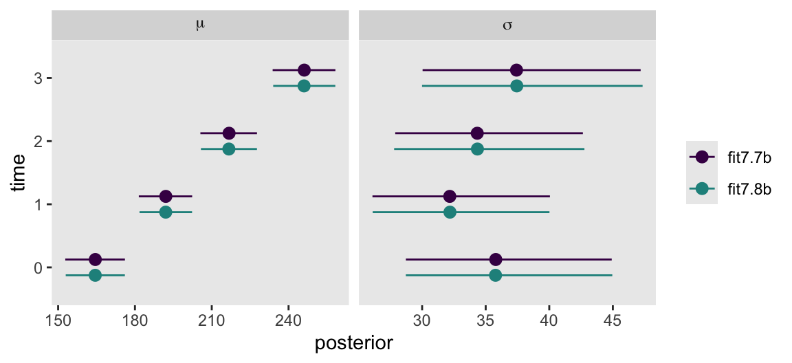
This time, let’s just compare the \(\mu\) and \(\sigma\) posteriors in a coefficient plot.

# combine
bind_rows(
  as_draws_df(fit7.7b) %>%
    select(contains("factortime")) %>% 
    set_names(c(str_c("mu_", 0:3), str_c("sigma_", 0:3))),
  as_draws_df(fit7.8b) %>%
    select(starts_with("b_"), starts_with("sigma_"))  %>% 
    set_names(c(str_c("mu_", 0:3), str_c("sigma_", 0:3)))
) %>% 
  # wrangle
  mutate(fit = rep(c("fit7.7b", "fit7.8b"), each = n() / 2)) %>% 
  pivot_longer(-fit) %>% 
  separate(name, into = c("par", "time"), sep = "_") %>% 
  group_by(fit, par, time) %>% 
  mean_qi(value) %>%
  
  # plot!
  ggplot(aes(x = value, xmin = .lower, xmax = .upper, y = time, group = fit, color = fit)) +
  geom_pointrange(position = position_dodge(width = -0.5)) +
  scale_color_viridis_d(NULL, end = 0.5) +
  xlab("posterior") +
  facet_wrap(~ par, labeller = label_parsed, scales = "free_x") +
  theme(panel.grid = element_blank())

Now the results between the two methods are very similar. If you wanted to, you could make a similar kind of plot for the two versions of the correlation matrix, too. Thus, the various models Singer and Willett introduced in this chapter are special multivariate alternatives to the standard multilevel approach we’ve preferred up to this point. Cool, huh?

Session info

sessionInfo()
R version 4.5.1 (2025-06-13)
Platform: aarch64-apple-darwin20
Running under: macOS Ventura 13.4

Matrix products: default
BLAS:   /Library/Frameworks/R.framework/Versions/4.5-arm64/Resources/lib/libRblas.0.dylib 
LAPACK: /Library/Frameworks/R.framework/Versions/4.5-arm64/Resources/lib/libRlapack.dylib;  LAPACK version 3.12.1

locale:
[1] en_US.UTF-8/en_US.UTF-8/en_US.UTF-8/C/en_US.UTF-8/en_US.UTF-8

time zone: America/Chicago
tzcode source: internal

attached base packages:
[1] stats     graphics  grDevices utils     datasets  methods   base     

other attached packages:
 [1] tidybayes_3.0.7 brms_2.23.0     Rcpp_1.1.0      lubridate_1.9.4 forcats_1.0.1   stringr_1.6.0   dplyr_1.1.4    
 [8] purrr_1.2.1     readr_2.1.5     tidyr_1.3.2     tibble_3.3.1    ggplot2_4.0.1   tidyverse_2.0.0

loaded via a namespace (and not attached):
 [1] svUnit_1.0.8            tidyselect_1.2.1        viridisLite_0.4.2       farver_2.1.2            loo_2.9.0.9000         
 [6] S7_0.2.1                fastmap_1.2.0           TH.data_1.1-4           tensorA_0.36.2.1        digest_0.6.39          
[11] estimability_1.5.1      timechange_0.3.0        lifecycle_1.0.5         StanHeaders_2.36.0.9000 survival_3.8-3         
[16] magrittr_2.0.4          posterior_1.6.1.9000    compiler_4.5.1          rlang_1.1.7             tools_4.5.1            
[21] utf8_1.2.6              knitr_1.51              labeling_0.4.3          bridgesampling_1.2-1    htmlwidgets_1.6.4      
[26] bit_4.6.0               pkgbuild_1.4.8          curl_7.0.0              plyr_1.8.9              RColorBrewer_1.1-3     
[31] abind_1.4-8             multcomp_1.4-29         withr_3.0.2             grid_4.5.1              stats4_4.5.1           
[36] xtable_1.8-4            inline_0.3.21           emmeans_1.11.2-8        scales_1.4.0            MASS_7.3-65            
[41] cli_3.6.5               mvtnorm_1.3-3           rmarkdown_2.30          crayon_1.5.3            generics_0.1.4         
[46] RcppParallel_5.1.11-1   rstudioapi_0.17.1       reshape2_1.4.5          tzdb_0.5.0              rstan_2.36.0.9000      
[51] splines_4.5.1           bayesplot_1.15.0.9000   parallel_4.5.1          matrixStats_1.5.0       vctrs_0.7.0            
[56] V8_8.0.1                Matrix_1.7-3            sandwich_3.1-1          jsonlite_2.0.0          arrayhelpers_1.1-0     
[61] hms_1.1.4               bit64_4.6.0-1           ggdist_3.3.3            glue_1.8.0              codetools_0.2-20       
[66] distributional_0.5.0    stringi_1.8.7           gtable_0.3.6            QuickJSR_1.8.1          pillar_1.11.1          
[71] htmltools_0.5.9         Brobdingnag_1.2-9       R6_2.6.1                vroom_1.6.6             evaluate_1.0.5         
[76] lattice_0.22-7          backports_1.5.0         rstantools_2.5.0.9000   coda_0.19-4.1           gridExtra_2.3          
[81] nlme_3.1-168            checkmate_2.3.3         xfun_0.55               zoo_1.8-14              pkgconfig_2.0.3        

Comments